Google Sheets – TheAppsScriptLab

10 Practical Google Sheets Tips

Posted on December 11, 2025by lidia.calicia@gmail.com

Here are 10 Google Sheets tips I use in my day-to-day.
You might recognise a few of them, but I’m pretty confident you’ll still learn something new!

Highlight an entire row based on a single cell

One of the most common questions:
“I want the whole row to change color when the status is ‘Done’ / the date is today / the checkbox is ticked.”

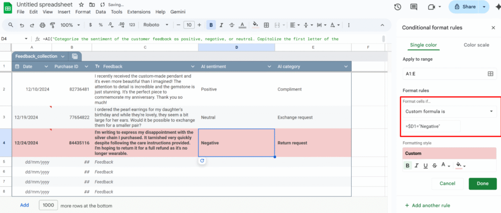
Example: highlight every review row where column D is "Negative".

1 – Open Conditional format rules (Format > Conditional formatting)

2 – Select the range you want to format, e.g. A1:E1000.

3 – Under “Format rules”, choose “Custom formula is“

4 – Insert the formula:

=$D1="Negative"

5 – Choose your formatting style and click Done.

Because the range starts at row 1, the formula uses =$D1. If your range starts at row 2 (for example, you skipped the header row), you’d use:

=$D2="Negative"

Use checkboxes to drive your formatting and logic

You can use checkboxes as a simple “on/off” switch to control formatting.

Example: highlight the entire row when the checkbox in column F is checked.

Format → Conditional formatting → Custom formula is:

Insert checkboxes in A1:F1000

Select the range to format, e.g. A1:F1000.

=$F1=true

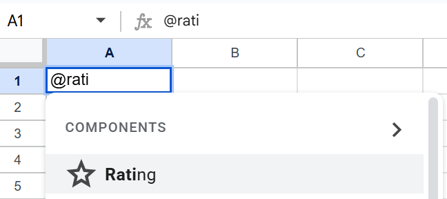
Turn ratings into a quick dropdown (@rating)

If you want fast feedback in a sheet (for tasks, clients, content, etc.), convert a column into a simple rating system.

With the Rating smart chip (@rating):

In a cell, type @rating and insert the Rating component.
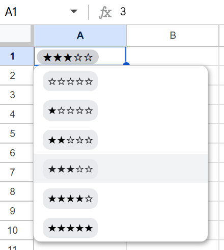
It creates a small star-based rating widget you can click to set the score.

You now have:

A consistent rating scale across your sheet.
An easy way to scan what’s high/low rated at a glance.
A clean input that still behaves like a value you can reference in formulas or filters.

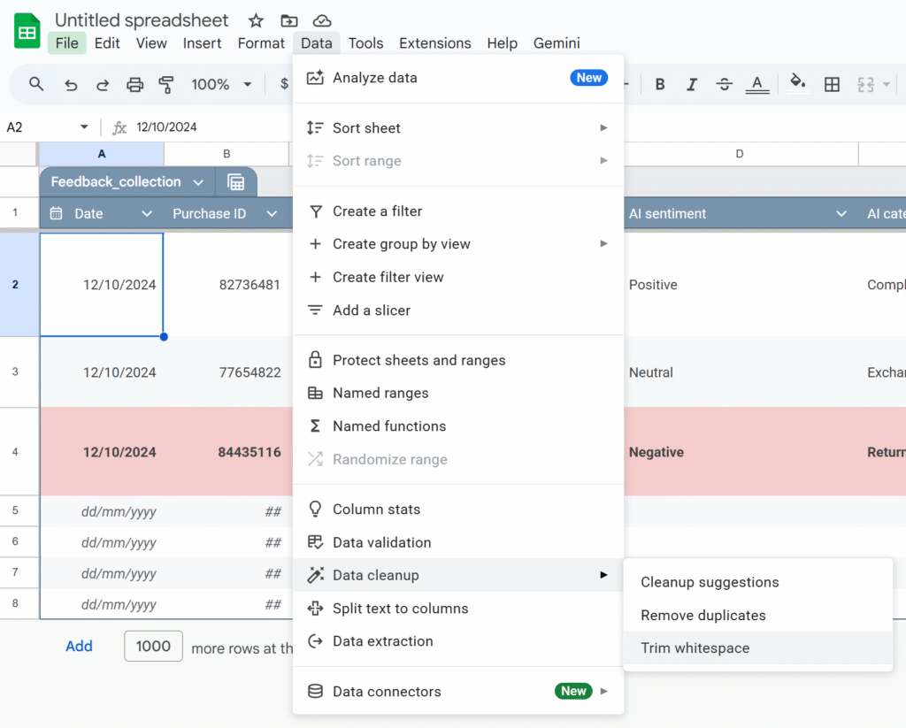
Use Data cleanup

Imported data is messy: extra spaces, duplicates, weird values. Google added built-in cleanup tools that are massively underused.

Cleanup suggestions: A sidebar proposes actions: remove duplicates, fix inconsistent capitalization, etc.

Remove duplicates: You choose the columns to check; Sheets shows how many duplicates it found and removes them.

Trim whitespace: This fixes issues where "ABC" and "ABC " look the same but don’t match in formulas.

Run these before you start building formulas. It saves a lot of debugging time later.

Stop dragging formulas: use ARRAYFORMULA

Common spreadsheet horror story: “My new rows don’t have the formula”, or “someone overwrote a formula with a value”.

ARRAYFORMULA lets you write the formula once and apply it to the whole column.

Example: instead of this in E2:

=B2*C2

and dragging it down, use:

=ARRAYFORMULA(
  IF(
    B2:B="",
    ,
    B2:B * C2:C
  )
)

This:

Applies the multiplication to every row where column B is not empty.
Automatically covers new rows as you add data.
Reduces the risk of someone “breaking” a single cell formula in the middle of your column.

Split CSV-style data into columns (without formulas)

If you’ve ever:

Pasted CSV data into column A,
Used =SPLIT() everywhere,
Then deleted column A manually…

You don’t have to.

Use Data → Split text to columns:

Paste the raw data into one column.
Select that column.
Go to Data → Split text to columns.
Choose the separator (comma, semicolon, space, custom, etc.).

Sheets automatically splits your data into multiple columns without formulas.

Use QUERY instead of copy-pasting filtered tables

Instead of manually filtering and copy-pasting, use QUERY and FILTER to build live views of your data.

Example: from a master task sheet (Sheet4!A1:E), create a separate view with only “To Do” tasks assigned to the person in G2:

=QUERY(
  Sheet4!A1:E,
  "select A, B, C, D, E 
   where C = 'To Do' 
   and D = '" & G2 & "'
   order by A",
  1
)

Whenever the main sheet is updated, this view updates automatically, no manual copy-paste needed.

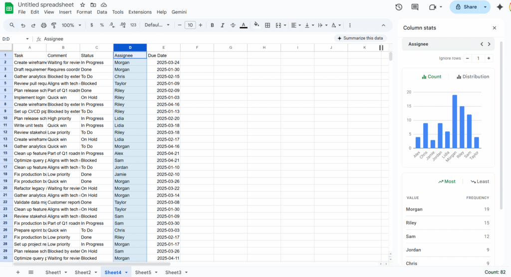
Use column stats to extract quickly key info

If you need a quick snapshot of what’s inside a column—value distribution, most common entries, min/max, etc.—use Column stats.

Right-click a column header.
Select Column stats.

You’ll get:

A count of unique values.
Basic stats (for numbers).
A small chart showing frequency by value.

Store phone numbers and IDs as text (so Sheets doesn’t “fix” them)

Sheets tries to be clever with numbers, which is bad news for things like phone numbers and IDs:

Leading zeros get removed.
Long IDs may be turned into scientific notation.

Best practices:

Set the column to Plain text:
Format → Number → Plain text.
Enter numbers with a leading apostrophe: '0412 345 678
Do the same for anything that looks numeric but isn’t a real “number”: phone numbers, SKUs, customer IDs, etc.

This prevents silent changes that are hard to detect later.

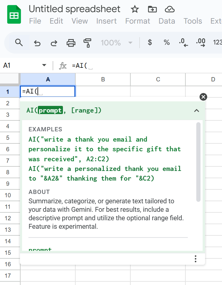
Prompt Gemini directly in your Sheets

Google Sheets now has a native AI function (often exposed as =AI() or =GEMINI(), depending on your Workspace rollout) that lets you talk directly to Google’s Gemini model from a cell.

Instead of nesting complex formulas, you can write natural-language prompts like:

=AI("Summarize this text in 3 bullet points:", A2)

You can use it to:

Summarize long text.
Classify or tag entries.
Extract key information from a sentence.
Generate content (subject lines, slogans, short paragraphs).

Because the prompt and the reference (like A2) live right in the formula, you can apply AI logic across a whole column just like any other function—without touching Apps Script or external tools.

If anything’s missing from this list, tell me! I’d love to hear your favourite Sheets tips and ideas.

Build Your Google Sheets Like React Components (with Apps Script)

Posted on December 5, 2025by lidia.calicia@gmail.com

Faster dashboards, cleaner code, and a rendering engine powered by the Sheets API.

Google Sheets is fantastic for quick dashboards, tracking tools, and prototypes. And with Apps Script, you can make them dynamic, automated, and even smarter.

But the moment you start building something real, a complex layout, a styled dashboard, a multi-section report, the Apps Script code quickly turns into:

messy
repetitive
slow
painful to maintain

Setting backgrounds, borders, number formats, writing values… everything requires individual calls, and your script balloon quickly.

To make this easier, you usually have two options:

Inject data into an existing template
Or…using RenderSheet

RenderSheet is a tiny, component-based renderer for Google Sheets, inspired by React’s architecture and built entirely in Apps Script.
Let’s explore how it works.!

Introducing RenderSheet

RenderSheet is a lightweight, React-inspired renderer for Google Sheets.

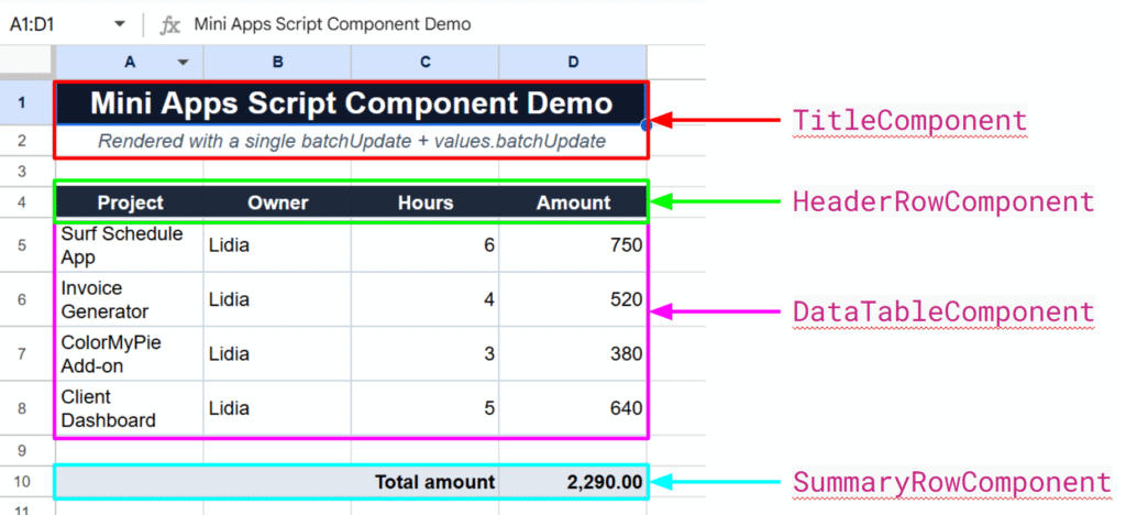
Instead of scattering .setValue(), .setBackground(), .setFontWeight(), etc. everywhere in your script, you write components:

<Title />
<HeaderRow />
<DataTable />
<SummaryRow />
<StatusPill />, etc.

Each component knows how to render itself.
Your spreadsheet becomes a clean composition of reusable blocks, just like a frontend UI.

Why a “React-like” approach?

React works because it forces you to think in components:

a Header component
a Table component
a Summary component
a StatusPill component

Each component knows how to render itself, and the app becomes a composition of smaller reusable pieces.I wanted the exact same thing, but for spreadsheets.

With RenderSheet, instead of writing:

sheet.getRange("A1").setValue("Hello");
sheet.getRange("A1").setBackground("#000");
sheet.getRange("A1").setFontWeight("bold");
// and so on...

You write:

class HeaderComponent extends SheetComponent {
  render() {
    this.context.writeRange("Sheet1!A1", [["Hello"]]);
    this.context.setBackground("Sheet1", "A1", "#000");
  }
}

No direct API calls. No multiple setValue() calls.
Just a clean render() method.

The Core Idea: One Render = Two Sheets API Calls

To achieve this “single render” effect, we simply divide to conquer:

one API call for injecting the data

and another for applying all the styling

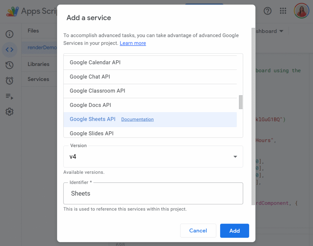
Before we can make the magic happen, we need to enable the Advanced Google Sheets API in our Apps Script project.
This unlocks the batchUpdate method, the real engine behind RenderSheet.

To do so, just click the little + button on the left side panel, in front of Services, and select Google Sheets API:

This gives you access to the batchUpdate method, the real engine behind RenderSheet.

Now let’s look at the core mechanism.

The SheetContext (the Render Engine)

SheetContext is the core of RenderSheet.
It collects all writes and formatting instructions and applies them in two API calls, using easy functions such as:

all data writes (writeRange)
all formatting instructions (setBackground, setTextFormat, setAlignment…)

But here’s the key:

None of these functions execute anything immediately.
They only describe what the component wants to render.

The actual rendering only happens at the end, through two API calls.

You can think of SheetContext as your “toolbox”, and feel free to extend it with your own helpers.

Here is its full implementation:

class SheetContext {
  constructor(spreadsheetId) {
    this.spreadsheetId = spreadsheetId;
    this.valueRanges = [];
    this.requests = [];
  }

  writeRange(rangeA1, values) {
    this.valueRanges.push({ range: rangeA1, values });
  }

  setBackground(sheetName, a1Range, color) {
    const gridRange = this.convertA1ToGridRange(sheetName, a1Range);
    if (!gridRange) return;

    this.requests.push({
      repeatCell: {
        range: gridRange,
        cell: { userEnteredFormat: { backgroundColor: this.hexToRgbColor(color) }},
        fields: "userEnteredFormat.backgroundColor",
      },
    });
  }

  setNumberFormat(sheetName, a1Range, numberFormatPattern) {
    const gridRange = this.convertA1ToGridRange(sheetName, a1Range);
    if (!gridRange) return;

    this.requests.push({
      repeatCell: {
        range: gridRange,
        cell: {
          userEnteredFormat: {
            numberFormat: { type: "NUMBER", pattern: numberFormatPattern },
          },
        },
        fields: "userEnteredFormat.numberFormat",
      },
    });
  }

  setTextFormat(sheetName, a1Range, options) {
    const gridRange = this.convertA1ToGridRange(sheetName, a1Range);
    if (!gridRange) return;

    const textFormat = {};
    if (options.bold !== undefined) textFormat.bold = options.bold;
    if (options.italic !== undefined) textFormat.italic = options.italic;
    if (options.underline !== undefined) textFormat.underline = options.underline;
    if (options.fontSize !== undefined) textFormat.fontSize = options.fontSize;
    if (options.color) {
      textFormat.foregroundColor = this.hexToRgbColor(options.color);
    }

    this.requests.push({
      repeatCell: {
        range: gridRange,
        cell: { userEnteredFormat: { textFormat }},
        fields: "userEnteredFormat.textFormat",
      },
    });
  }

  setAlignment(sheetName, a1Range, options) {
    const gridRange = this.convertA1ToGridRange(sheetName, a1Range);
    if (!gridRange) return;

    const format = {};
    const fields = [];

    if (options.horizontal) {
      format.horizontalAlignment = options.horizontal;
      fields.push("userEnteredFormat.horizontalAlignment");
    }
    if (options.vertical) {
      format.verticalAlignment = options.vertical;
      fields.push("userEnteredFormat.verticalAlignment");
    }

    this.requests.push({
      repeatCell: {
        range: gridRange,
        cell: { userEnteredFormat: format },
        fields: fields.join(","),
      },
    });
  }

  setWrapStrategy(sheetName, a1Range, wrapStrategy) {
    const gridRange = this.convertA1ToGridRange(sheetName, a1Range);
    if (!gridRange) return;

    this.requests.push({
      repeatCell: {
        range: gridRange,
        cell: { userEnteredFormat: { wrapStrategy }},
        fields: "userEnteredFormat.wrapStrategy",
      },
    });
  }

  setBorders(sheetName, a1Range, options) {
    const gridRange = this.convertA1ToGridRange(sheetName, a1Range);
    if (!gridRange) return;

    const border = {
      style: options.style || "SOLID",
      width: options.width || 1,
      color: options.color ? this.hexToRgbColor(options.color) : undefined,
    };

    this.requests.push({
      updateBorders: {
        range: gridRange,
        top: border,
        bottom: border,
        left: border,
        right: border,
        innerHorizontal: border,
        innerVertical: border,
      },
    });
  }

  mergeRange(sheetName, a1Range, mergeType) {
    const gridRange = this.convertA1ToGridRange(sheetName, a1Range);
    if (!gridRange) return;

    this.requests.push({
      mergeCells: {
        range: gridRange,
        mergeType: mergeType || "MERGE_ALL",
      },
    });
  }

  unmergeRange(sheetName, a1Range) {
    const gridRange = this.convertA1ToGridRange(sheetName, a1Range);
    if (!gridRange) return;

    this.requests.push({ unmergeCells: { range: gridRange }});
  }

  autoResizeColumns(sheetName, a1Range) {
    const gridRange = this.convertA1ToGridRange(sheetName, a1Range);
    if (!gridRange) return;

    this.requests.push({
      autoResizeDimensions: {
        dimensions: {
          sheetId: gridRange.sheetId,
          dimension: "COLUMNS",
          startIndex: gridRange.startColumnIndex,
          endIndex: gridRange.endColumnIndex,
        },
      },
    });
  }

  setDataValidationList(sheetName, a1Range, values) {
    const gridRange = this.convertA1ToGridRange(sheetName, a1Range);
    if (!gridRange || values.length === 0) return;

    this.requests.push({
      setDataValidation: {
        range: gridRange,
        rule: {
          condition: {
            type: "ONE_OF_LIST",
            values: values.map(v => ({ userEnteredValue: v })),
          },
          showCustomUi: true,
        },
      },
    });
  }

  addRequest(request) {
    this.requests.push(request);
  }

  commit() {
    if (this.requests.length > 0) {
      Sheets.Spreadsheets.batchUpdate(
        { requests: this.requests },
        this.spreadsheetId
      );
    }

    if (this.valueRanges.length > 0) {
      Sheets.Spreadsheets.Values.batchUpdate(
        { valueInputOption: "USER_ENTERED", data: this.valueRanges },
        this.spreadsheetId
      );
    }
  }

  hexToRgbColor(hex) {
    let clean = hex.replace("#", "");
    if (clean.length === 3) {
      clean = clean.split("").map(ch => ch + ch).join("");
    }
    return {
      red: parseInt(clean.substring(0, 2), 16) / 255,
      green: parseInt(clean.substring(2, 4), 16) / 255,
      blue: parseInt(clean.substring(4, 6), 16) / 255,
    };
  }

  convertA1ToGridRange(sheetName, a1Range) {
    const ss = SpreadsheetApp.openById(this.spreadsheetId);
    const sheet = ss.getSheetByName(sheetName);
    if (!sheet) throw new Error(`Sheet not found: ${sheetName}`);

    const range = sheet.getRange(a1Range);
    return {
      sheetId: sheet.getSheetId(),
      startRowIndex: range.getRow() - 1,
      endRowIndex: range.getRow() - 1 + range.getNumRows(),
      startColumnIndex: range.getColumn() - 1,
      endColumnIndex: range.getColumn() - 1 + range.getNumColumns(),
    };
  }
}

The SheetComponent (your building block)

If SheetContext is the engine, SheetComponent is the UI framework you build with.

Components never call the Sheets API themselves.
They only describe what they want through this.context.

class SheetComponent {
  constructor(context, props) {
    this.context = context;
    this.props = props || {};
  }

  render() {
    // To be overridden
  }

  renderChild(ComponentClass, props) {
    const child = new ComponentClass(this.context, props);
    child.render();
    return child;
  }
}

This gives you:

clean reusable components
predictable rendering
composition (just like React)

Example:

class StatusPill extends SheetComponent {
  render() {
    const { sheetName, range, status } = this.props;

    const color =
      status === "Done" ? "#10b981" :
      status === "Blocked" ? "#ef4444" :
      "#facc15";

    this.context.setBackground(sheetName, range, color);
    this.context.setTextFormat(sheetName, range, { bold: true, color: "#fff" });
    this.context.setAlignment(sheetName, range, { horizontal: "CENTER" });
  }
}

An easy example of use

Let’s build a tiny dashboard using:

TitleComponent
HeaderRowComponent
DataTableComponent
SummaryRowComponent

Each is a simple SheetComponent that writes values and applies styles using this.context.

**
 * Component that writes a big title and optional subtitle at the top.
 */
class TitleComponent extends SheetComponent {

  render() {
    const sheetName = (this.props.sheetName);
    const title = (this.props.title);
    const subtitle = (this.props.subtitle);

    this.context.writeRange(`${sheetName}!A1`, [[title]]);
    this.context.mergeRange(sheetName, "A1:D1", "MERGE_ALL");
    this.context.setBackground(sheetName, "A1:D1", "#0f172a");
    this.context.setTextFormat(sheetName, "A1:D1", {
      bold: true,
      fontSize: 16,
      color: "#ffffff",
    });
    this.context.setAlignment(sheetName, "A1:D1", { horizontal: "CENTER", vertical: "MIDDLE" });

    if (subtitle) {
      this.context.writeRange(`${sheetName}!A2`, [[subtitle]]);
      this.context.mergeRange(sheetName, "A2:D2", "MERGE_ALL");
      this.context.setTextFormat(sheetName, "A2:D2", {
        italic: true,
        color: "#475569",
      });
      this.context.setAlignment(sheetName, "A2:D2", { horizontal: "CENTER", vertical: "MIDDLE" });
    }
  }
}

/**
 * Component that writes a header row with styling.
 */
class HeaderRowComponent extends SheetComponent {
  /**
   * @returns {void}
   */
  render() {
    const sheetName = (this.props.sheetName);
    const headers = (this.props.headers);
    const rowIndex = (this.props.rowIndex);

    const lastColLetter = columnIndexToLetter(headers.length);
    const rangeA1 = `${sheetName}!A${rowIndex}:${lastColLetter}${rowIndex}`;

    this.context.writeRange(rangeA1, [headers]);
    this.context.setBackground(sheetName, `A${rowIndex}:${lastColLetter}${rowIndex}`, "#1e293b");
    this.context.setTextFormat(sheetName, `A${rowIndex}:${lastColLetter}${rowIndex}`, {
      bold: true,
      color: "#ffffff",
    });
    this.context.setAlignment(sheetName, `A${rowIndex}:${lastColLetter}${rowIndex}`, {
      horizontal: "CENTER",
      vertical: "MIDDLE",
    });
  }
}

/**
 * Component that writes a 2D data table starting at a given row.
 */
class DataTableComponent extends SheetComponent {
  /**
   * @returns {void}
   */
  render() {
    const sheetName = (this.props.sheetName);
    const rows = (this.props.rows);
    const startRow = (this.props.startRow);

    if (!rows || rows.length === 0) return;

    const numCols = rows[0].length;
    const lastColLetter = columnIndexToLetter(numCols);
    const endRow = startRow + rows.length - 1;
    const rangeA1 = `${sheetName}!A${startRow}:${lastColLetter}${endRow}`;

    this.context.writeRange(rangeA1, rows);
    this.context.setBorders(sheetName, `A${startRow}:${lastColLetter}${endRow}`, {
      style: "SOLID",
      width: 1,
      color: "#cbd5e1",
    });
    this.context.setAlignment(sheetName, `A${startRow}:${lastColLetter}${endRow}`, {
      vertical: "MIDDLE",
    });
    this.context.setWrapStrategy(sheetName, `A${startRow}:${lastColLetter}${endRow}`, "WRAP");
  }
}

class SummaryRowComponent extends SheetComponent {
  /**
   * @returns {void}
   */
  render() {
    const sheetName = (this.props.sheetName);
    const label = (this.props.label);
    const rowIndex = (this.props.rowIndex);
    const numCols = (this.props.numCols);
    const amountColumnIndex = (this.props.amountColumnIndex);

    const lastColLetter = columnIndexToLetter(numCols);
    const labelCell = `A${rowIndex}`;
    const amountCell = `${columnIndexToLetter(numCols)}${rowIndex}`;
    const labelRangeSingle = `${sheetName}!${labelCell}`;
    const fullRowRange = `A${rowIndex}:${lastColLetter}${rowIndex}`;
    const amountRange = `${sheetName}!${amountCell}`;

    // Write label in a single cell only
    this.context.writeRange(labelRangeSingle, [[label]]);

    // Then merge the label area visually
    this.context.mergeRange(
      sheetName,
      `A${rowIndex}:${columnIndexToLetter(numCols - 1)}${rowIndex}`,
      "MERGE_ALL"
    );

    this.context.setAlignment(sheetName, fullRowRange, {
      horizontal: "RIGHT",
      vertical: "MIDDLE",
    });
    this.context.setBackground(sheetName, fullRowRange, "#e2e8f0");
    this.context.setTextFormat(sheetName, fullRowRange, {
      bold: true,
    });

    const dataStartRow = (this.props.dataStartRow);
    const dataEndRow = (this.props.dataEndRow);
    const amountColLetter = columnIndexToLetter(amountColumnIndex);
    const sumFormula = `=SUM(${amountColLetter}${dataStartRow}:${amountColLetter}${dataEndRow})`;

    this.context.writeRange(amountRange, [[sumFormula]]);
    this.context.setNumberFormat(sheetName, amountCell, "#,##0.00");
  }
}

Now let’s assemble everything inside a root component:

/**
 * Root dashboard component that composes title, headers, data and summary.
 */
class DemoDashboardComponent extends SheetComponent {

  render() {
    const sheetName = (this.props.sheetName);
    const headers = (this.props.headers);
    const rows = (this.props.rows);

    this.renderChild(TitleComponent, {
      sheetName,
      title: "Mini Apps Script Component Demo",
      subtitle: "Rendered with a single batchUpdate + values.batchUpdate",
    });

    const headerRowIndex = 4;
    this.renderChild(HeaderRowComponent, {
      sheetName,
      headers,
      rowIndex: headerRowIndex,
    });

    const dataStartRow = headerRowIndex + 1;
    this.renderChild(DataTableComponent, {
      sheetName,
      rows,
      startRow: dataStartRow,
    });

    const dataEndRow = dataStartRow + rows.length - 1;
    const summaryRowIndex = dataEndRow + 2;

    this.renderChild(SummaryRowComponent, {
      sheetName,
      label: "Total amount",
      rowIndex: summaryRowIndex,
      numCols: headers.length,
      amountColumnIndex: headers.length,
      dataStartRow,
      dataEndRow,
    });

    const lastColLetter = columnIndexToLetter(headers.length);
    this.context.autoResizeColumns(sheetName, `A1:${lastColLetter}${summaryRowIndex}`);
  }
}

Here’s a screenshot of the spreadsheet output, where you can see how each component contributes to the final layout:

Rendering the dashboard:

/**
 * Entry point: renders a full demo dashboard using the component system.
 *
 * @returns {void}
 */
function renderDemoDashboard() {
  const ss = SpreadsheetApp.openById("1mRno9TPj1iXGQ_lEqBIy3jOz4tyJm6upsVhklGuG1BQ")
  const spreadsheetId = ss.getId();
  const sheetName = "Demo";
  const headers = ["Project", "Owner", "Hours", "Amount"];
  const rows = [
    ["Surf Schedule App", "Lidia", 6, 750],
    ["Invoice Generator", "Lidia", 4, 520],
    ["ColorMyPie Add-on", "Lidia", 3, 380],
    ["Client Dashboard", "Lidia", 5, 640],
  ];

  renderSheet(spreadsheetId, DemoDashboardComponent, {
    sheetName,
    headers,
    rows,
  });
}

Even though the initial setup is a bit more structured, the final result:

renders in 1 second
stays perfectly maintainable
allows components to be reused in any dashboard

Exactly the power of React, but in Google Sheets.

Final Thoughts

RenderSheet brings structure, speed, and clarity to Google Sheets development.
If you’re tired of repetitive formatting code or want to build Sheets dashboards the same way you build UIs, this pattern completely changes the experience.

Let me know what you think, and feel free to contribute!

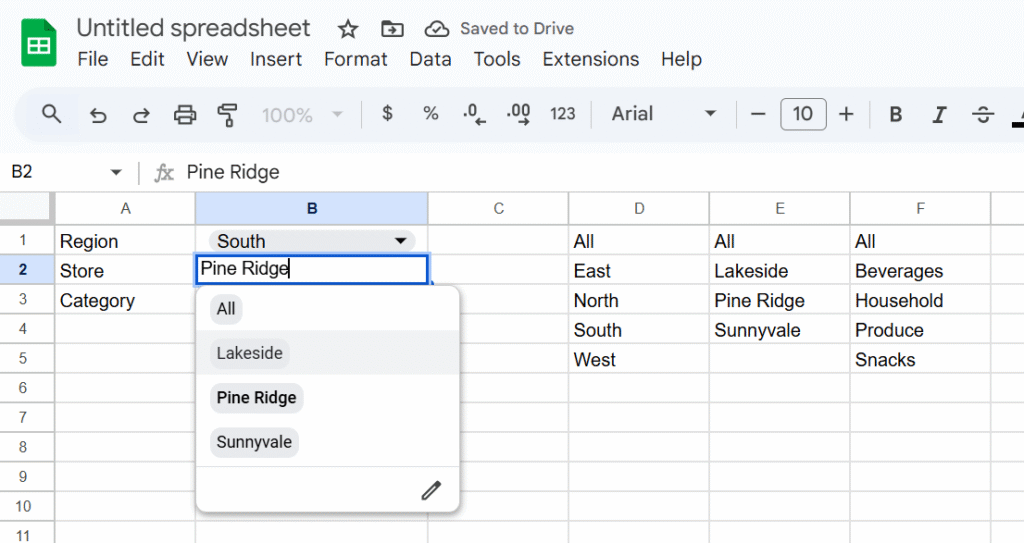
Filter by a Dropdown in Google Sheets (Data Validation + QUERY)

Posted on November 11, 2025by lidia.calicia@gmail.com

Dashboards feel magical when they react instantly to a selection, no scripts, no reloads, just smooth changes as you click a dropdown.

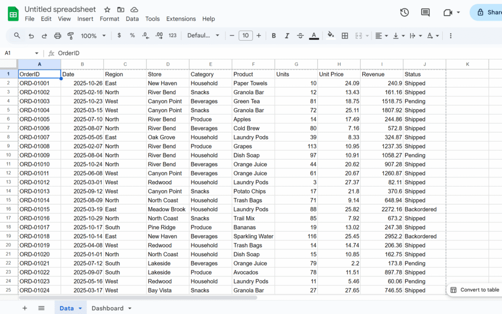
In this tutorial, we will build exactly that in Google Sheets: pick a Region, optionally refine by Store and Category, and watch your results table update in real time. We’ll use built-in tools, Data validation for dropdowns and QUERY for the live results, so it’s fast, maintainable, and friendly for collaborators.

In this example, we’ll use a sales dataset and create dropdowns for Region, Store, and Category, but you can easily adapt the approach to your own data and fields.

Step 1 – Add control labels

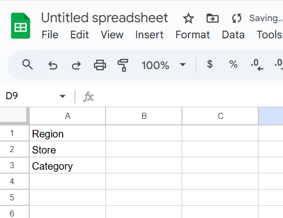
Let’s create a sheet, named Dashbaord, and add

A1: Region

A2: Store (dependent on Region)

A3: Category

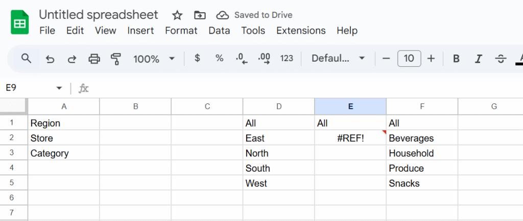
Step 2 – Build dynamic lists (helper formulas)

In column D, we will create a dynamic list of region with the following formula (insert the formula in D1):

={"All"; SORT(UNIQUE(FILTER(Data!C2:C, Data!C2:C<>"")))}

In column E, we will create a depending list for stores (changes when store update)

={"All";
  IF(Dashboard!B1="All",
     SORT(UNIQUE(FILTER(Data!D2:D, Data!D2:D<>""))),
     SORT(UNIQUE(FILTER(Data!D2:D, Data!C2:C=Dashboard!B1)))
  )
}

And in column F, the products

={"All"; SORT(UNIQUE(FILTER(Data!E2:E, Data!E2:E<>"")))}

Why formulas instead of manual lists? They stay in sync when new rows arrive.

Step 3 — Create the dropdowns (Data → Data validation)

B1 (Region): List from a range → Dashboard!D1:D

B2 (Store): List from a range → Dashboard!D2:D

B3 (Category): List from a range → Dashboard!D3:D
Enable “Show dropdown” and set “Reject input” to avoid typos.

Step 4 — Place the QUERY result table

Pick a location for your live table—let’s use Dashboard!A5. Paste this formula:

=QUERY(
  Data!A1:J,
  "select * where (" &
    "(Col3 = '"&SUBSTITUTE(B1,"'","''")&"' or '"&B1&"'='All') and " &
    "(Col4 = '"&SUBSTITUTE(B2,"'","''")&"' or '"&B2&"'='All') and " &
    "(Col5 = '"&SUBSTITUTE(B3,"'","''")&"' or '"&B3&"'='All')" &
  ")",
  1
)

How it works

The source range Data!A1:J sets column numbers for QUERY:
- Col3 = Region, Col4 = Store, Col5 = Category.
Each condition allows “All” to match everything.
SUBSTITUTE(...,"'","''") safely escapes values like O'Brien.

If your headers aren’t in row 1, change the last parameter (1) to the correct header row count or adjust the range.

Hope this walkthrough helped! If there’s another Sheets topic you’d like me to cover, drop it in the comments.

Calling the Sheets API from a Library

Posted on September 29, 2025by lidia.calicia@gmail.com

One of the common traps with Apps Script libraries is when the library uses an Advanced Google Service (like the Sheets API).
Even if the logic lives in the library, the calling script must also enable and authorize the same service.

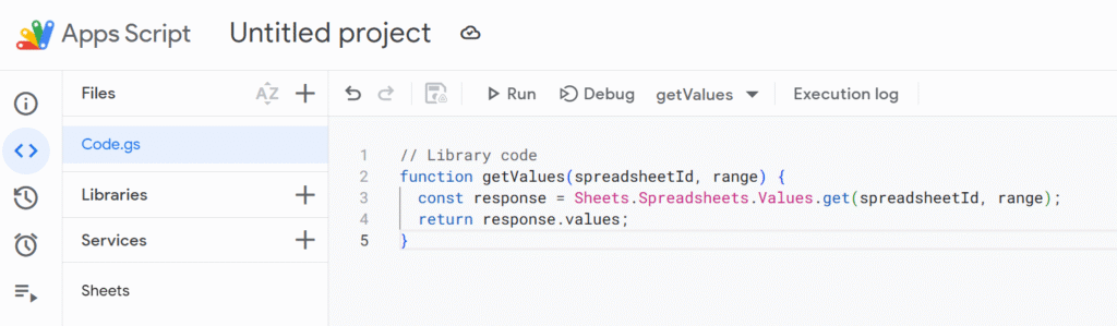
1. Library Project

Let’s say you create a project called SheetsHelper.
It has one function to read sheet values using the Advanced Sheets API:

// Library code
function getValues(spreadsheetId, range) {
  const response = Sheets.Spreadsheets.Values.get(spreadsheetId, range);
  return response.values;
}

This uses the Sheets API, not the simpler SpreadsheetApp. This service needs to be enabled manually from the left side panel in the Apps Script UI.

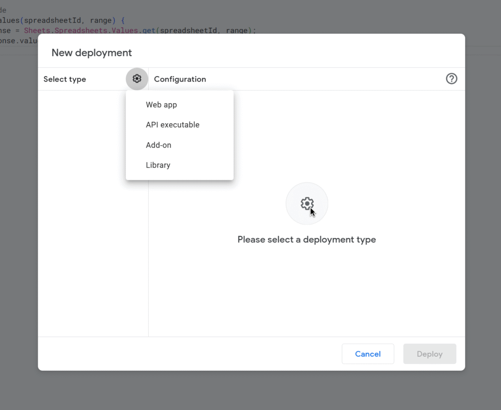
2. Deploy the Library

Save your project.
Go to File > Project properties > Script ID, copy the ID.
In your target script, go to Services > Libraries, paste the Script ID, and give it a name like SheetsHelper.

3. Calling Script

Now in another project you call your newly deployed library:

function testLibrary() {
  const ssId = SpreadsheetApp.getActiveSpreadsheet().getId();
  const data = SheetsHelper.getValues(ssId, "Sheet1!A1:C5");
  Logger.log(data);
}

Sheets service must also be enabled in the calling script. Otherwise, this will throw an error.

Apps Script libraries don’t run in isolation.
The execution environment is always the calling script.
That means:

Scopes are declared in the caller’s appsscript.json.
Advanced Services must be enabled in the caller’s project.
Authorizations are stored per user + calling project, not in the library.

The library is just code, the permissions live in the project that calls it.

When using a library that depends on APIs, you must configure the calling project with the same advanced settings. Libraries don’t transfer authorizations — they only share code.

How to Create Dependent Drop-Down Lists in Google Sheets (Dynamic Cascading Drop-Downs)

Posted on September 28, 2025by lidia.calicia@gmail.com

Google Sheets drop-downs are a great way to control inputs and keep your data clean. A classic use case is to have different options for a drop down, depending on what was selecting in another.

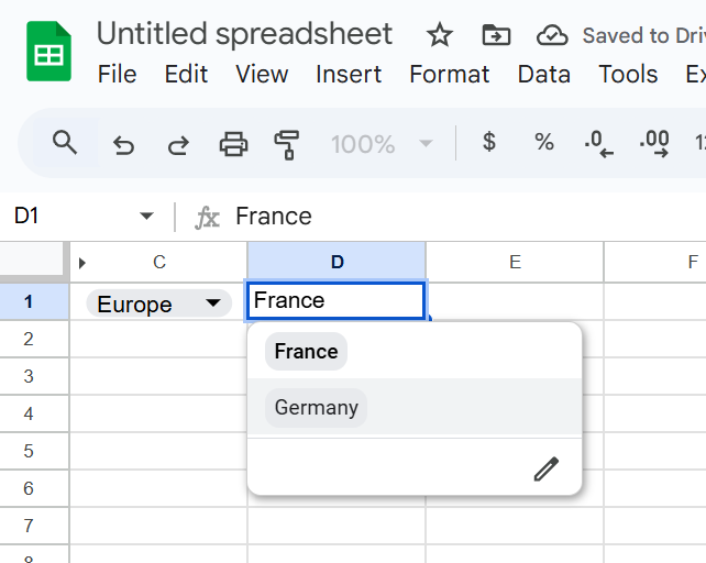
That’s where dependent drop-down lists (also called cascading drop-downs) come in. For example:

In Drop-Down 1, you select a Region (Europe, Asia, America).
In Drop-Down 2, you only see the Countries from that region (Europe → France, Germany, Spain).

This guide shows you step by step how to build dependent drop-downs in Google Sheets — without named ranges, using formulas and a simple script for better usability.

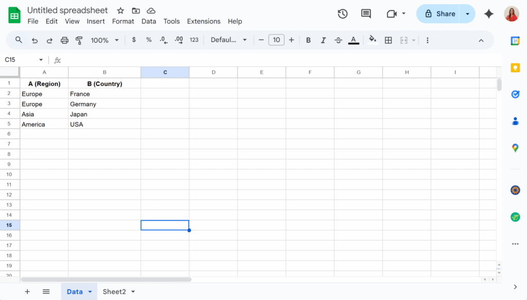
Step 1 – Organize your source data

On a sheet named Data, enter your list in two columns:

Important: Use one row per country (don’t put “France, Germany, Spain” in a single cell).

Step 2 – Create the drop-down lists

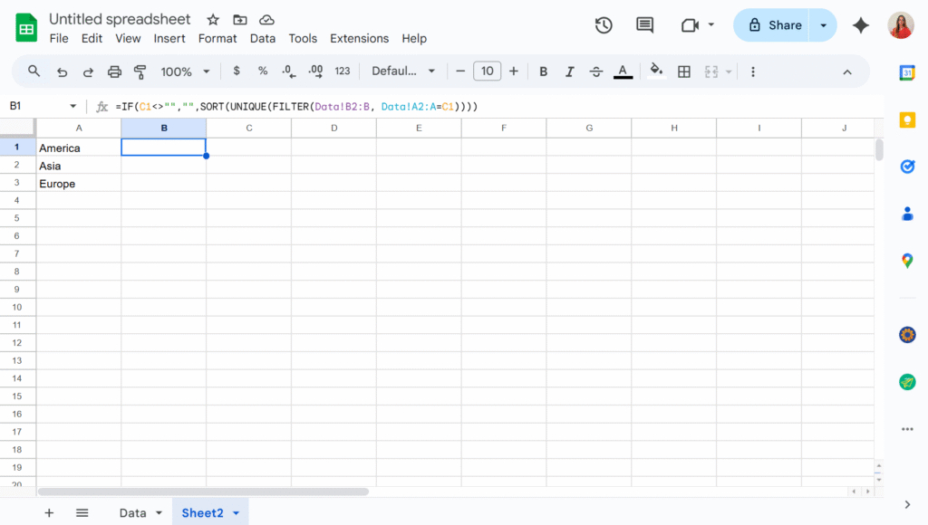
The key is not to link drop-downs directly to your raw lists, but to use formulas that generate the lists dynamically. These formulas can live on the same sheet as your data or on a separate one. In this example, I’ll place them in Sheet2 to keep the Data sheet uncluttered.

In A2, I will add the formula:

=SORT(UNIQUE(FILTER(Data!A2:A, Data!A2:A<>"")))

This way, the first drop-down will display a clean list of countries without any duplicates.

And in B2, assuming the country drop-down will be in C1 :

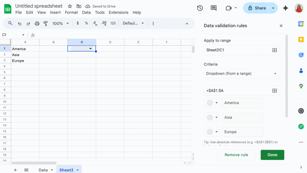
=IF(C1<>"","",SORT(UNIQUE(FILTER(Data!B2:B, Data!A2:A=C1))))

Step 3 – Create the drop-down

Now we can simply add two drop-downs in C1 and D1, using the “Dropdown from a range” option in the Data validation menu.

The second drop-down will now display only the values that match the selection from the first drop-down. You can then hide columns A and B to keep your sheet tidy — and voilà!