Conditional Formatting in Google Sheets (Simple Guide)

Conditional formatting in Google Sheets is one of the easiest ways to make your data more readable and actionable. Instead of manually styling cells, you can automatically apply formatting based on rules.
Want to:

  • Highlight values greater than 10
  • Bold rows where status is “On going” and due date is today
  • Instantly visualize trends

Conditional formatting handles all of that.
In this guide, you’ll learn the most useful techniques to master conditional formatting in Google Sheets.

How to add a conditional formatting rule in Google Sheets

To create a rule:

  • Select your data range
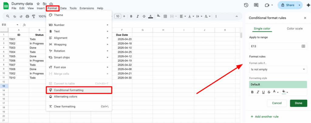
  • Go to Format → Conditional formatting
  • The sidebar opens on the right, where you configure your rule
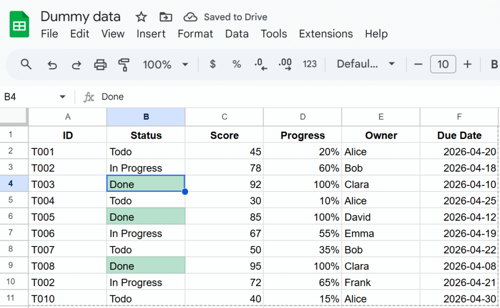
Let’s start with a simple example: highlight all statuses marked as “Done”.
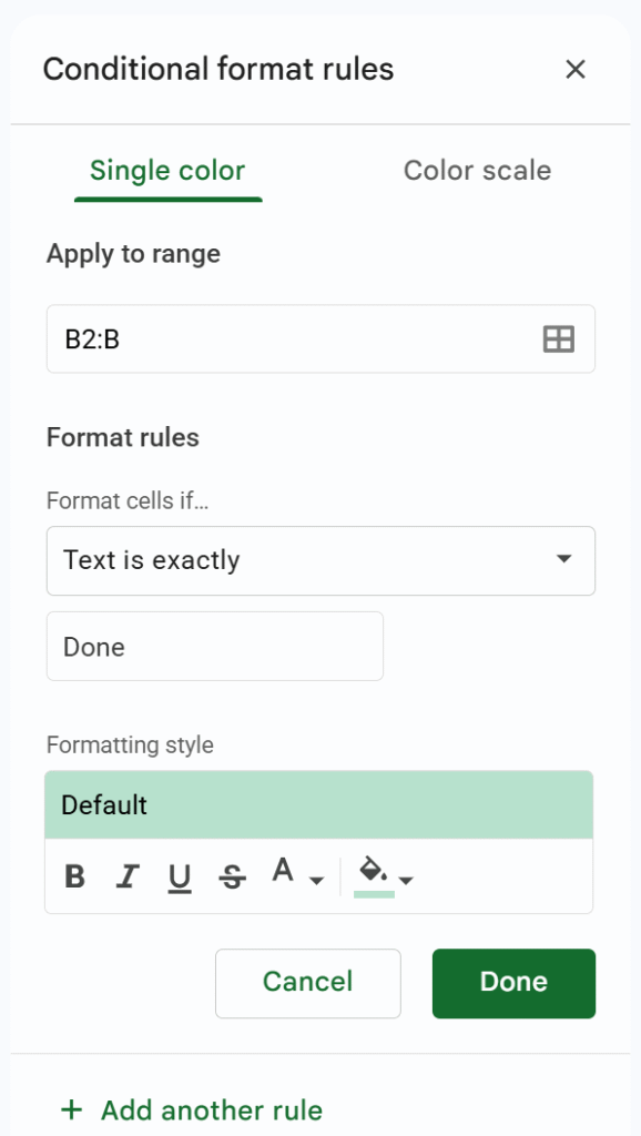
  • Range: B2:B (this excludes headers and automatically includes new rows)
  • Rule: Text is exactly → "Done"
  • Formatting style: green background (you can also change text color, bold, etc.)
Apply conditional formatting to an entire row (custom formula)

In most cases, formatting a single cell is not enough. You often want to highlight the entire row based on a condition.

To do this, use a custom formula.
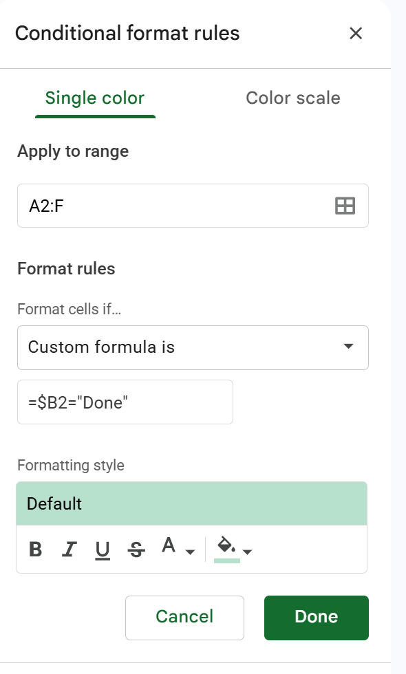
  • Range: select your full dataset (e.g. A2:E)
  • Format rule: Custom formula is
  • Formula:
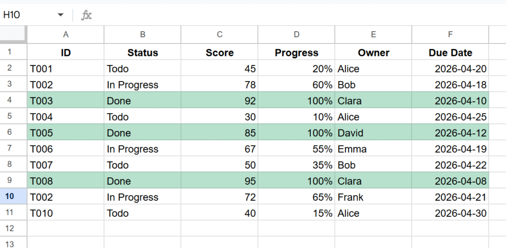
=$B2="Done"

    This formula checks column B (status), and if the value is “Done”, the formatting is applied to the entire row.
    Use color scale for quick visual analysis

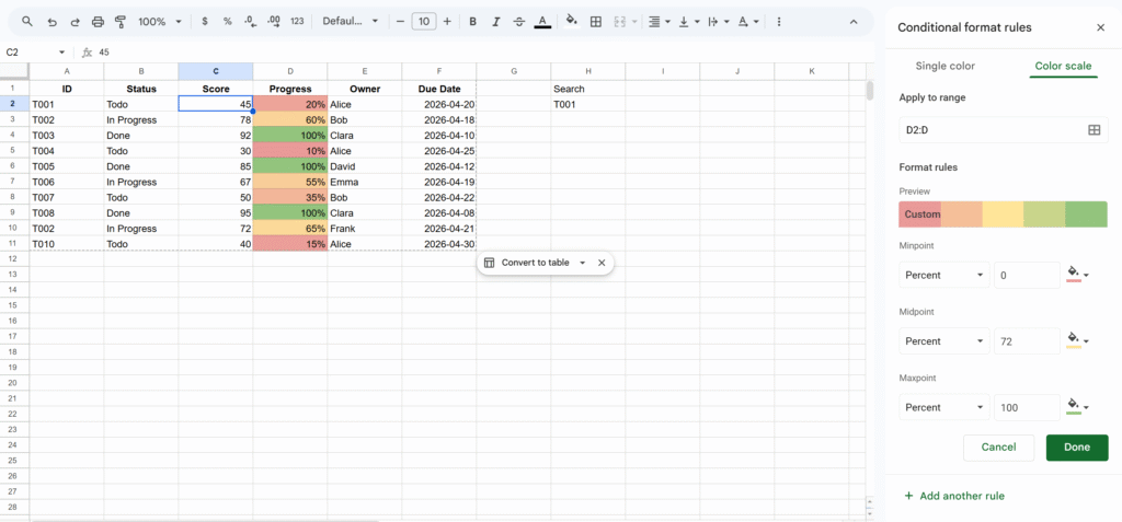
    The color scale feature lets you apply a gradient based on numeric values.
    You can access it from the second tab in the conditional formatting panel.
    You can configure:

    • The color gradient (low → high)
    • Minimum, midpoint, and maximum values
    • The type of values (number, percent, percentile)
    Tip: Highlight duplicates in Google Sheets

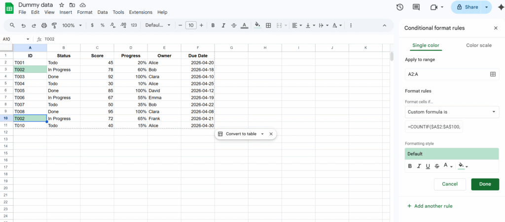
    A very common use case is detecting duplicates.

    You can do this using a custom formula:

    =COUNTIF($A$2:$A$100, A2) > 1
    Tip: Format based on another cell

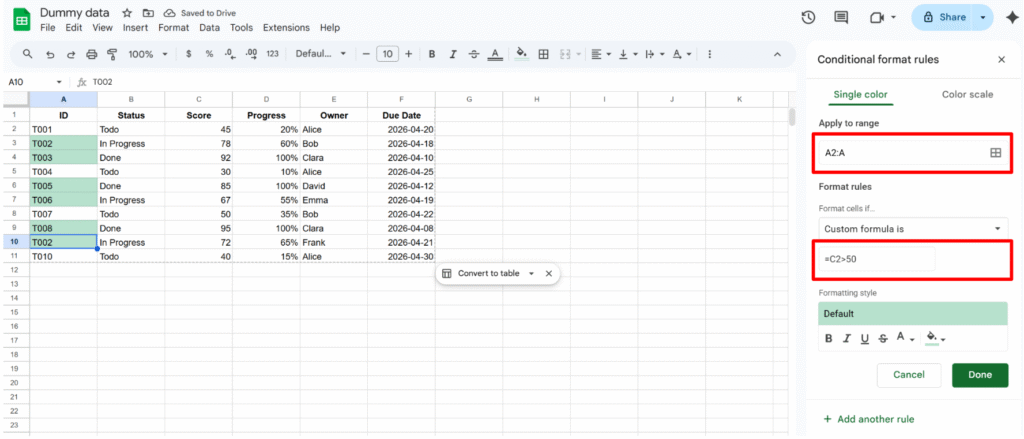
    Conditional formatting doesn’t have to depend on the same cell. You can apply formatting based on values in another column.

    For example, you can format column A depending on values in column B.

    This approach is widely used in:

    • Task trackers
    • Workflow systems
    • Status-based dashboards

    The key is to combine ranges + custom formulas.
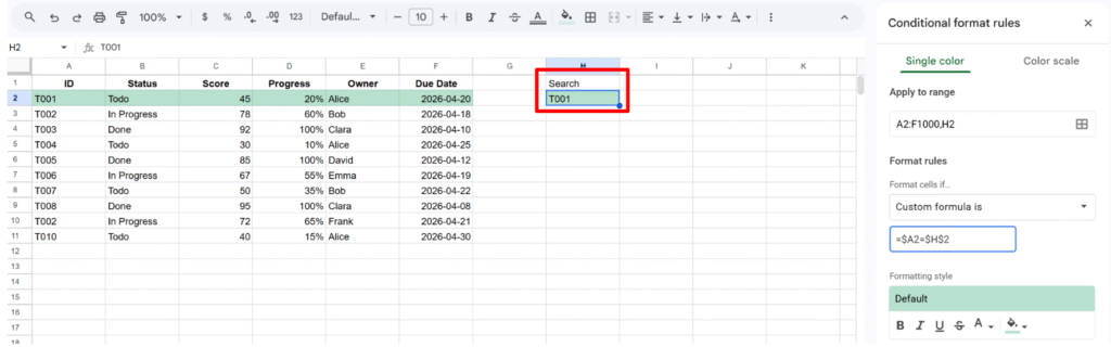
    Tip: Highlight a row based on search input

    You can also create a simple search experience directly in Google Sheets:

    =$A2=$H$2
    • Cell H2 acts as a search input
    • When you type a value, matching rows are highlighted

    This is very useful for:

    • Quick lookups
    • CRM systems
    • Large datasets navigation

    Final thoughts

    This is a good base to understand how conditional formatting works.
    Once you get the logic, you can easily adapt it to your own use cases and build more advanced rules.
    Filter by a Dropdown in Google Sheets (Data Validation + QUERY)

    Dashboards feel magical when they react instantly to a selection, no scripts, no reloads, just smooth changes as you click a dropdown.

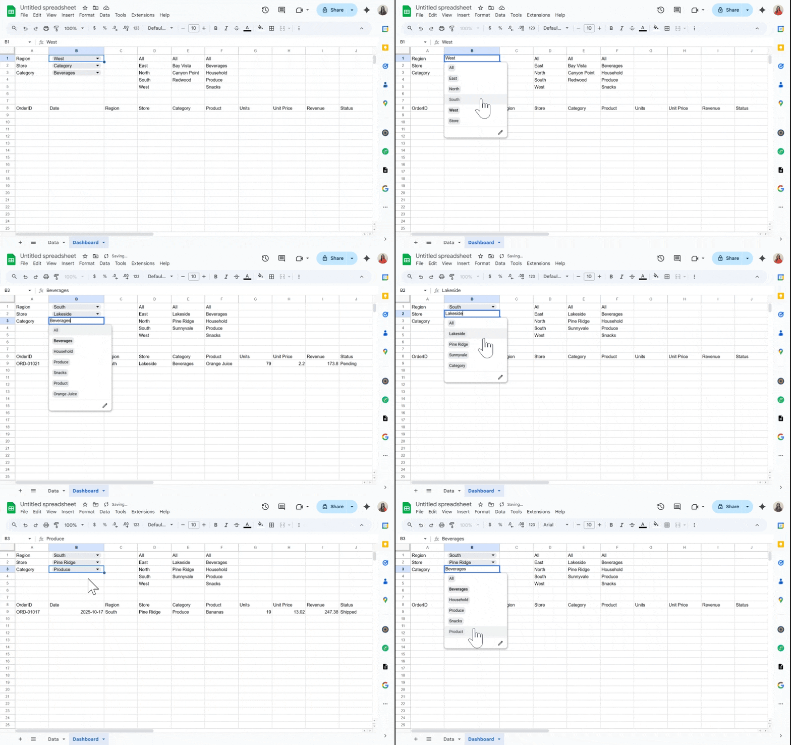
    In this tutorial, we will build exactly that in Google Sheets: pick a Region, optionally refine by Store and Category, and watch your results table update in real time. We’ll use built-in tools, Data validation for dropdowns and QUERY for the live results, so it’s fast, maintainable, and friendly for collaborators.

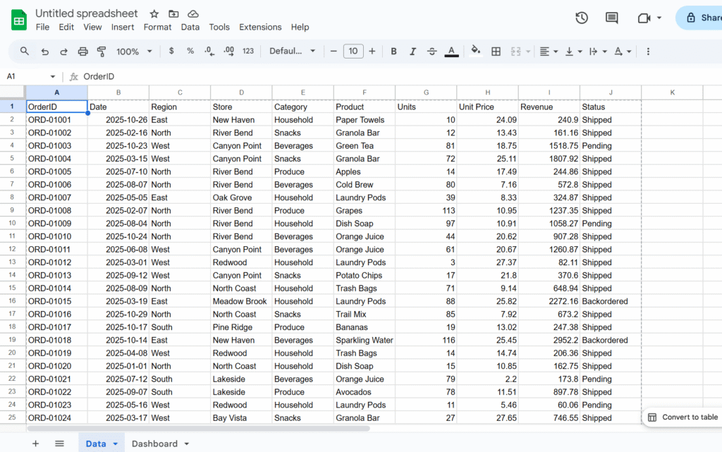
    In this example, we’ll use a sales dataset and create dropdowns for Region, Store, and Category, but you can easily adapt the approach to your own data and fields.

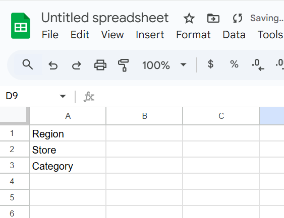
    Step 1 – Add control labels

    Let’s create a sheet, named Dashbaord, and add

    A1: Region

    A2: Store (dependent on Region)

    A3: Category

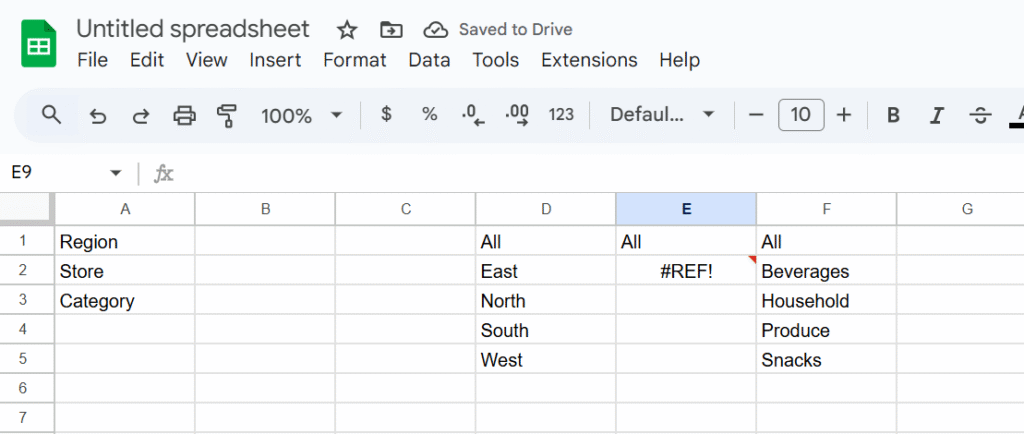
    Step 2 – Build dynamic lists (helper formulas)

    In column D, we will create a dynamic list of region with the following formula (insert the formula in D1):

    ={"All"; SORT(UNIQUE(FILTER(Data!C2:C, Data!C2:C<>"")))}

    In column E, we will create a depending list for stores (changes when store update)

    ={"All";
      IF(Dashboard!B1="All",
         SORT(UNIQUE(FILTER(Data!D2:D, Data!D2:D<>""))),
         SORT(UNIQUE(FILTER(Data!D2:D, Data!C2:C=Dashboard!B1)))
      )
    }

    And in column F, the products

    ={"All"; SORT(UNIQUE(FILTER(Data!E2:E, Data!E2:E<>"")))}

    Why formulas instead of manual lists? They stay in sync when new rows arrive.

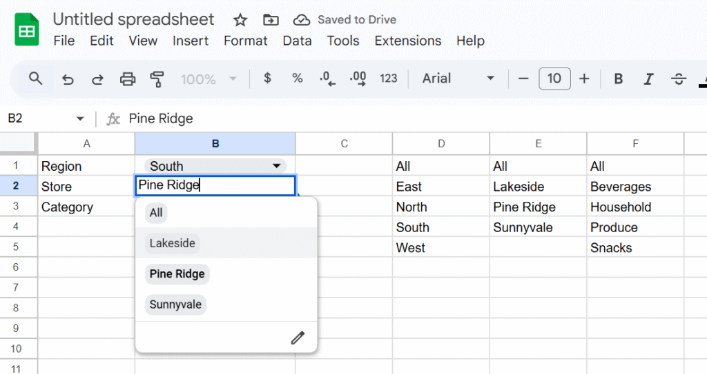
    Step 3 — Create the dropdowns (Data → Data validation)

    B1 (Region): List from a range → Dashboard!D1:D

    B2 (Store): List from a range → Dashboard!D2:D

    B3 (Category): List from a range → Dashboard!D3:D
    Enable “Show dropdown” and set “Reject input” to avoid typos.

    Step 4 — Place the QUERY result table

    Pick a location for your live table—let’s use Dashboard!A5. Paste this formula:

    =QUERY(
      Data!A1:J,
      "select * where (" &
        "(Col3 = '"&SUBSTITUTE(B1,"'","''")&"' or '"&B1&"'='All') and " &
        "(Col4 = '"&SUBSTITUTE(B2,"'","''")&"' or '"&B2&"'='All') and " &
        "(Col5 = '"&SUBSTITUTE(B3,"'","''")&"' or '"&B3&"'='All')" &
      ")",
      1
    )

    How it works

    • The source range Data!A1:J sets column numbers for QUERY:
      • Col3 = Region, Col4 = Store, Col5 = Category.
    • Each condition allows “All” to match everything.
    • SUBSTITUTE(...,"'","''") safely escapes values like O'Brien.

    If your headers aren’t in row 1, change the last parameter (1) to the correct header row count or adjust the range.

    Hope this walkthrough helped! If there’s another Sheets topic you’d like me to cover, drop it in the comments.

    How to Create Dependent Drop-Down Lists in Google Sheets (Dynamic Cascading Drop-Downs)

    Google Sheets drop-downs are a great way to control inputs and keep your data clean. A classic use case is to have different options for a drop down, depending on what was selecting in another.

    That’s where dependent drop-down lists (also called cascading drop-downs) come in. For example:

    • In Drop-Down 1, you select a Region (Europe, Asia, America).
    • In Drop-Down 2, you only see the Countries from that region (Europe → France, Germany, Spain).

    This guide shows you step by step how to build dependent drop-downs in Google Sheets — without named ranges, using formulas and a simple script for better usability.

    Step 1 – Organize your source data

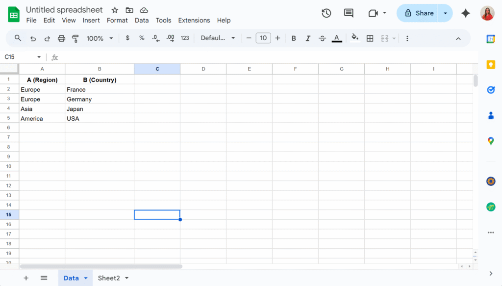
    On a sheet named Data, enter your list in two columns:

    Important: Use one row per country (don’t put “France, Germany, Spain” in a single cell).

    Step 2 – Create the drop-down lists

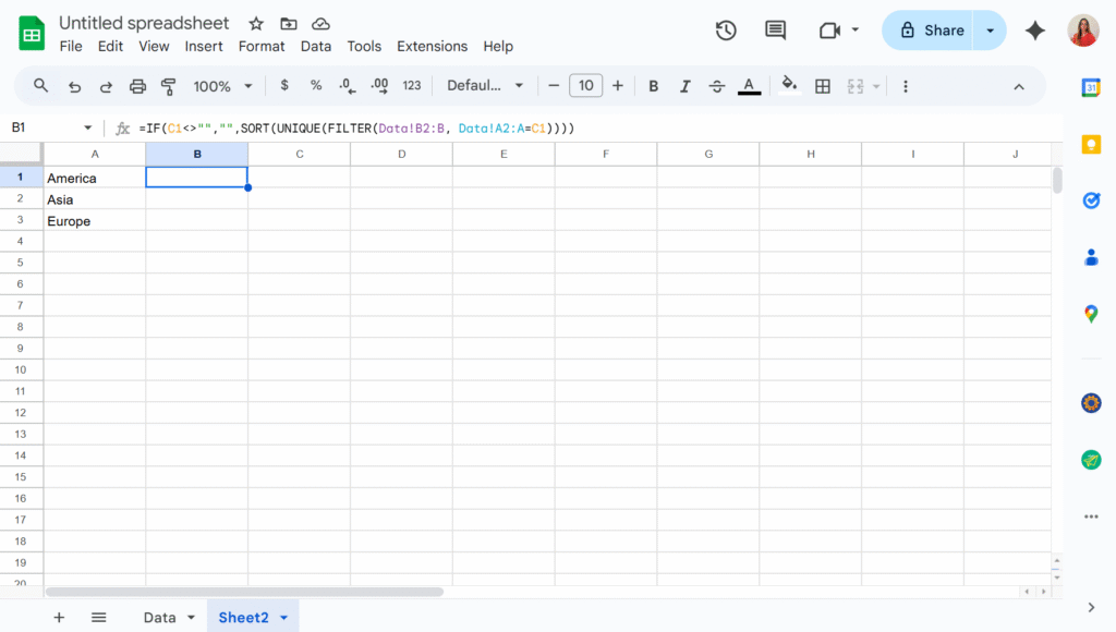
    The key is not to link drop-downs directly to your raw lists, but to use formulas that generate the lists dynamically. These formulas can live on the same sheet as your data or on a separate one. In this example, I’ll place them in Sheet2 to keep the Data sheet uncluttered.

    In A2, I will add the formula:

    =SORT(UNIQUE(FILTER(Data!A2:A, Data!A2:A<>"")))

    This way, the first drop-down will display a clean list of countries without any duplicates.

    And in B2, assuming the country drop-down will be in C1 :

    =IF(C1<>"","",SORT(UNIQUE(FILTER(Data!B2:B, Data!A2:A=C1))))

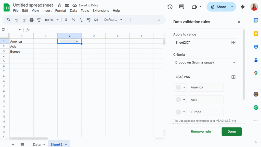
    Step 3 – Create the drop-down

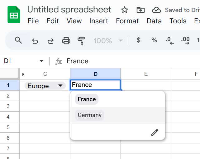
    Now we can simply add two drop-downs in C1 and D1, using the “Dropdown from a range” option in the Data validation menu.

    The second drop-down will now display only the values that match the selection from the first drop-down. You can then hide columns A and B to keep your sheet tidy — and voilà!