Google Sheets drop-downs are a great way to control inputs and keep your data clean. A classic use case is to have different options for a drop down, depending on what was selecting in another.
That’s where dependent drop-down lists (also called cascading drop-downs) come in. For example:
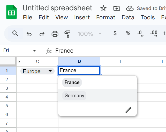
- In Drop-Down 1, you select a Region (Europe, Asia, America).
- In Drop-Down 2, you only see the Countries from that region (Europe → France, Germany, Spain).
This guide shows you step by step how to build dependent drop-downs in Google Sheets — without named ranges, using formulas and a simple script for better usability.
Step 1 – Organize your source data
On a sheet named Data, enter your list in two columns:
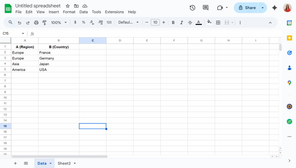
Important: Use one row per country (don’t put “France, Germany, Spain” in a single cell).
Step 2 – Create the drop-down lists
The key is not to link drop-downs directly to your raw lists, but to use formulas that generate the lists dynamically. These formulas can live on the same sheet as your data or on a separate one. In this example, I’ll place them in Sheet2 to keep the Data sheet uncluttered.
In A2, I will add the formula:
=SORT(UNIQUE(FILTER(Data!A2:A, Data!A2:A<>"")))This way, the first drop-down will display a clean list of countries without any duplicates.
And in B2, assuming the country drop-down will be in C1 :
=IF(C1<>"","",SORT(UNIQUE(FILTER(Data!B2:B, Data!A2:A=C1))))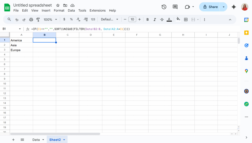
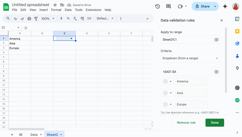
Step 3 – Create the drop-down
Now we can simply add two drop-downs in C1 and D1, using the “Dropdown from a range” option in the Data validation menu.
The second drop-down will now display only the values that match the selection from the first drop-down. You can then hide columns A and B to keep your sheet tidy — and voilà!