Conditional formatting in Google Sheets is one of the easiest ways to make your data more readable and actionable. Instead of manually styling cells, you can automatically apply formatting based on rules. Want to:
Highlight values greater than 10
Bold rows where status is “On going” and due date is today
Instantly visualize trends
Conditional formatting handles all of that. In this guide, you’ll learn the most useful techniques to master conditional formatting in Google Sheets.
How to add a conditional formatting rule in Google Sheets
To create a rule:
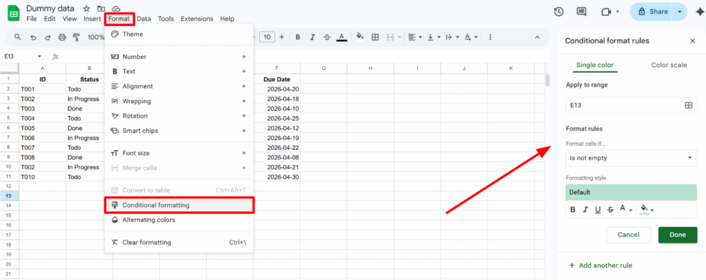
Select your data range
Go to Format → Conditional formatting
The sidebar opens on the right, where you configure your rule
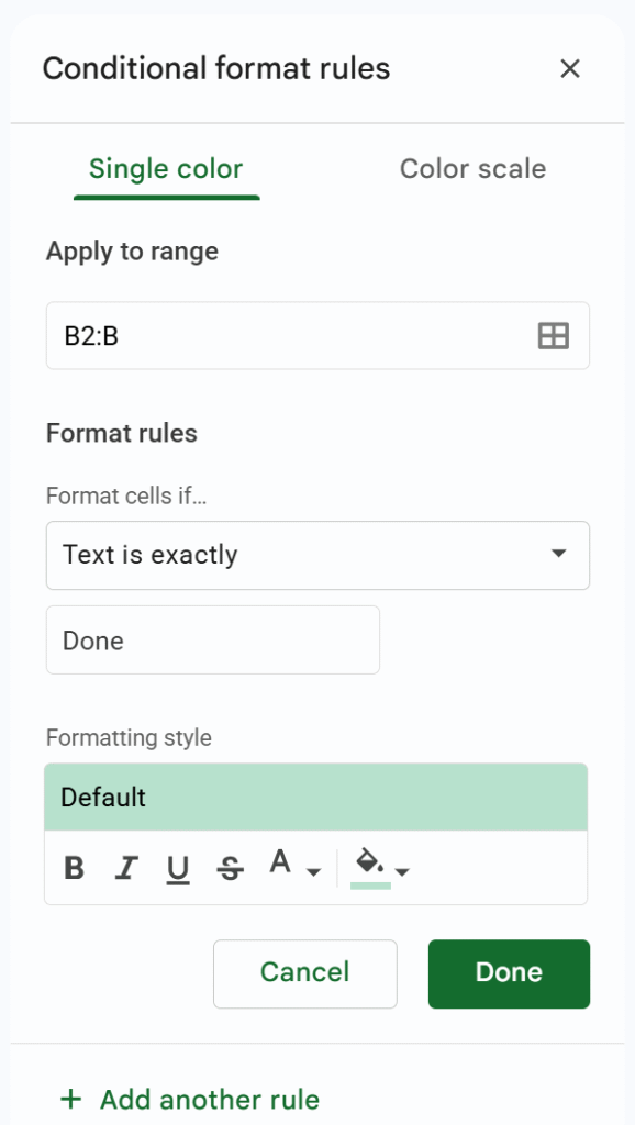
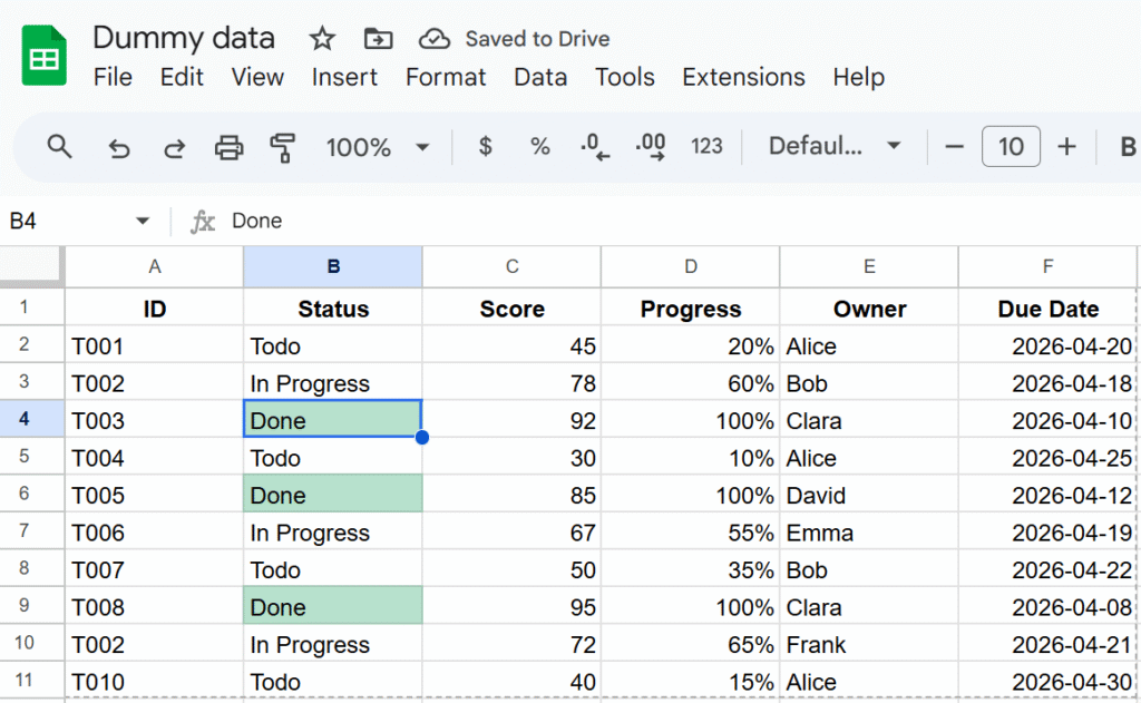
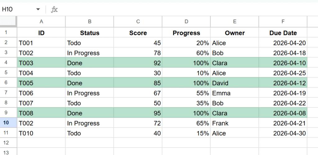
Let’s start with a simple example: highlight all statuses marked as “Done”.
Range: B2:B (this excludes headers and automatically includes new rows)
Rule:Text is exactly → "Done"
Formatting style: green background (you can also change text color, bold, etc.)
Apply conditional formatting to an entire row (custom formula)
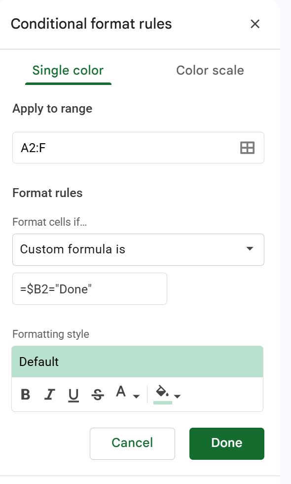
In most cases, formatting a single cell is not enough. You often want to highlight the entire row based on a condition.
To do this, use a custom formula.
Range: select your full dataset (e.g. A2:E)
Format rule:Custom formula is
Formula:
=$B2="Done"
This formula checks column B (status), and if the value is “Done”, the formatting is applied to the entire row.
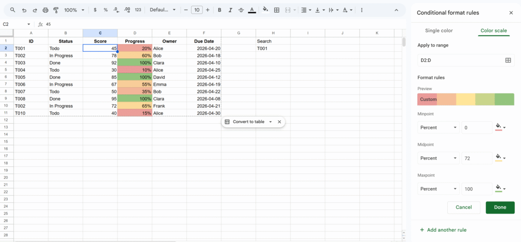
Use color scale for quick visual analysis
The color scale feature lets you apply a gradient based on numeric values. You can access it from the second tab in the conditional formatting panel. You can configure:
The color gradient (low → high)
Minimum, midpoint, and maximum values
The type of values (number, percent, percentile)
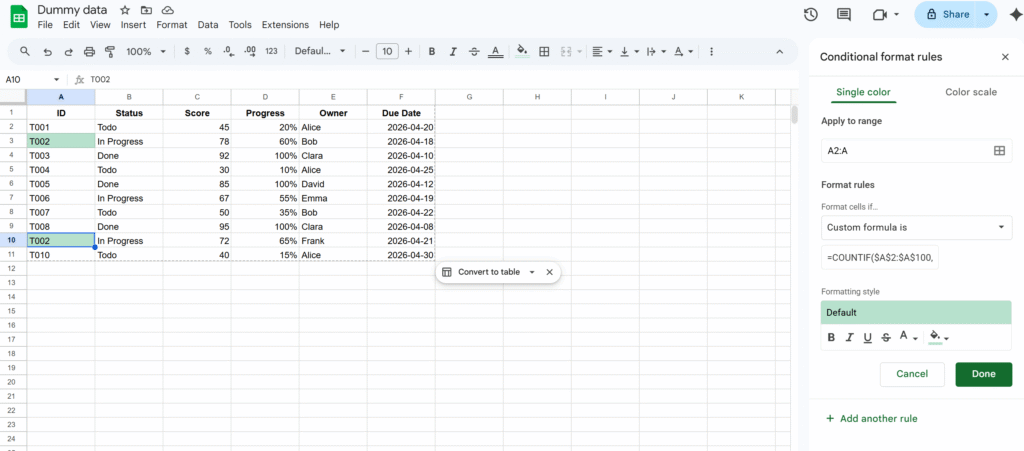
Tip: Highlight duplicates in Google Sheets
A very common use case is detecting duplicates.
You can do this using a custom formula:
=COUNTIF($A$2:$A$100, A2) > 1
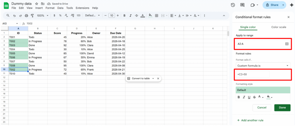
Tip: Format based on another cell
Conditional formatting doesn’t have to depend on the same cell. You can apply formatting based on values in another column.
For example, you can format column A depending on values in column B.
This approach is widely used in:
Task trackers
Workflow systems
Status-based dashboards
The key is to combine ranges + custom formulas.
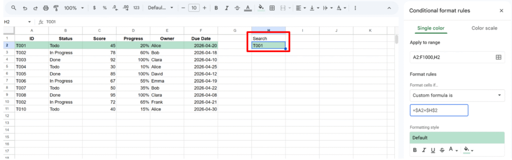
Tip: Highlight a row based on search input
You can also create a simple search experience directly in Google Sheets:
=$A2=$H$2
Cell H2 acts as a search input
When you type a value, matching rows are highlighted
This is very useful for:
Quick lookups
CRM systems
Large datasets navigation
Final thoughts
This is a good base to understand how conditional formatting works. Once you get the logic, you can easily adapt it to your own use cases and build more advanced rules.
When automating Google Sheets with Apps Script, two triggers are often confused: onEdit and onChange. They behave differently, and this short guide summarizes what actually triggers each one.
What triggers each event
Action in the spreadsheet
onEdit
onChange
Edit a cell value
✔️
✔️
Insert a row or column
❌
✔️
Delete a row or column
❌
✔️
Change background color or font
❌
✔️
Create or delete a sheet
❌
✔️
Move a column or row with data
✔️
✔️
Move a column or row without data
❌
✔️
Key idea
onEdit reacts to data edits inside cells.
onChange reacts to structural changes in the spreadsheet.
This means that formatting changes, sheet structure modifications, or column insertions will not trigger onEdit, but will trigger onChange.
Comparing the event objects
Another major difference is the object passed to the function.
Example: onEdit(e)
onEdit provides detailed information about the edited range.
When working with Google Forms + Google Sheets, a common setup is to connect several forms to the same spreadsheet. Each form creates its own response sheet automatically.
This works well at first. But as soon as you want to automate workflows with Google Apps Script, things become messy.
Typical situations:
You have multiple forms for different processes (client onboarding, support requests, event registrations, etc.)
Each form writes responses into a different sheet of the same spreadsheet
You want to trigger different automation logic depending on the form
The issue is that the Form Submit trigger in Google Sheets does not allow you to specify a different function depending on which form submitted the response.
The approach I use is to create one global trigger function that runs whenever a form submission occurs. This function then routes the event to the appropriate handler, based on the sheet that received the response.
A Single Dispatcher Trigger
The e object returned by the trigger provides the context of the event. From it, we can retrieve the range that triggered the execution, then access the sheet, and finally obtain the sheet name using function chaining.
const sheetName = e.range.getSheet().getName();
From there, we can decide which process should handle the submission.
Here is an example which can be easily
function Main_FormDispatcher(e) {

  // Get sheet name to retrieve what form was submitted
  const sheetName = e.range.getSheet().getName();

  Logger.log(`Form response received from sheet: ${sheetName}`);

  // Dispatch event
  if (sheetName === "Client Intake Responses") {
    processClientIntake(e);
  } else if (sheetName === "Bug Report Responses") {
    processBugReport(e);
  } else if (sheetName === "Newsletter Signup Responses") {
    processNewsletterSignup(e);
  } else {
    Logger.log(`Unknown form sheet detected: ${sheetName}`);
  }
}
If you regularly build Google Workspace automations, structuring your scripts around dispatcher functions like this one will save you a lot of time and complexity later.
If you use Xero and Google Sheets on a daily basis, this automation tutorial is for you. In this post, you’ll learn how to automatically sync your Xero bills into a Google Sheet on a schedule, so your spending table stays up to date without copy-pasting.
We’ll build it in a production-friendly way: OAuth2 authorization (so Xero can securely grant access), safe credential storage in Apps Script, a sync function that writes into your sheet, and refresh tokens (via offline_access) so the automation keeps running long-term.
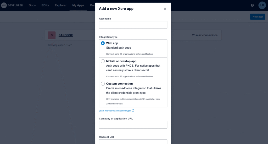
Create a Xero OAuth2 app
Create a Xero OAuth2 app in the Xero Developer portal and choose the web app / Standard auth code type (the standard flow Xero documents for third-party apps).The standard authorization code flow
The most important field is Redirect URI. Xero requires an exact, absolute redirect URI (no wildcards), so we will need the exact callback URL generated by your Apps Script project. Xero API – OAuth 2.0
Get a temporary redirect URI to create the app
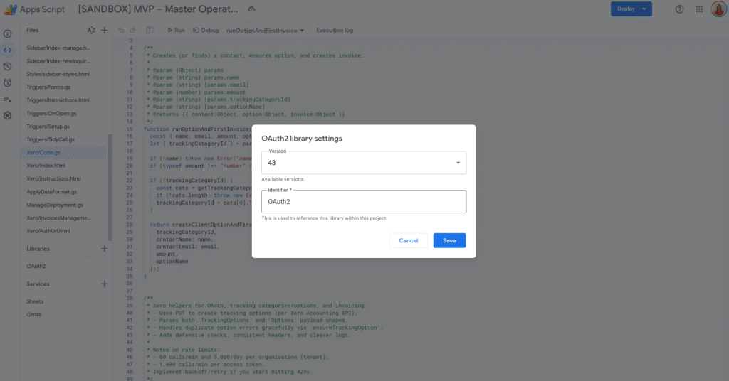
In Apps Script, the OAuth2 library can generate the exact redirect URI for this project. Run the function below, copy the URL from the logs, and paste it into your Xero app settings to finish creating the app.
/**
 * Logs the Redirect URI you must paste into your Xero app settings.
 * This does NOT require Client ID/Secret.
 *
 * @returns {void}
 */
function logXeroRedirectUri() {
  const service = OAuth2.createService('Xero')
    .setCallbackFunction('xeroAuthCallback');
  Logger.log(service.getRedirectUri());
}

/**
 * OAuth callback endpoint (stub is fine for this step).
 * @param {Object} e
 * @returns {GoogleAppsScript.HTML.HtmlOutput}
 */
function xeroAuthCallback(e) {
  return HtmlService.createHtmlOutput('Callback ready.');
}
The Apps Script OAuth2 library is the standard way to handle OAuth consent and token refresh in Apps Script. (Link to the setup guide here).
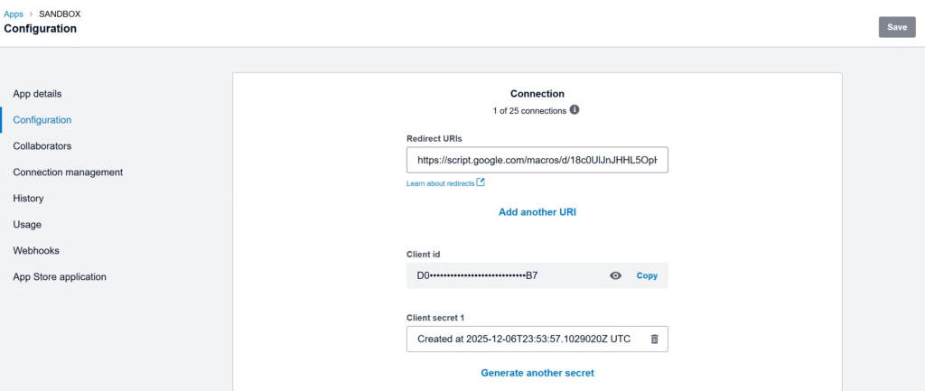
Get and store Client ID / Client Secret in Script Properties
Once the app is created, copy the Client ID and Client Secret. You’ll need them in Apps Script to complete the OAuth flow.
Store only the Client ID and Client Secret in Script Properties. OAuth tokens are user-specific, so we store them in User Properties via the OAuth2 library’s property store.
Replace the temporary callback with the real OAuth service + callback
Now that we have Client ID/Secret stored, we can build the real OAuth service and the real callback that stores tokens.
Important: tokens are user-specific, so we store them in User Properties via .setPropertyStore(PropertiesService.getUserProperties()).
Let’s replace the previous xeroAuthCallback() with this version:
/**
 * Creates and returns the OAuth2 service configured for Xero.
 * Client ID/Secret are in Script Properties; OAuth tokens are stored per-user in User Properties.
 *
 * @returns {OAuth2.Service}
 */
function getXeroService_() {
  const { clientId, clientSecret } = getXeroCredentials_();

  return OAuth2.createService('Xero')
    .setAuthorizationBaseUrl('https://login.xero.com/identity/connect/authorize')
    .setTokenUrl('https://identity.xero.com/connect/token')
    .setClientId(clientId)
    .setClientSecret(clientSecret)
    .setCallbackFunction('xeroAuthCallback')
    .setPropertyStore(PropertiesService.getUserProperties())
    .setCache(CacheService.getUserCache())
    .setLock(LockService.getUserLock())
    .setScope([
      'openid',
      'profile',
      'email',
      'offline_access',
      'accounting.transactions',
    ].join(' '))
    .setTokenHeaders({
      Authorization: 'Basic ' + Utilities.base64Encode(`${clientId}:${clientSecret}`),
    });
}

/**
 * OAuth callback endpoint called by Xero after consent.
 * This stores the access token + refresh token in the OAuth2 property store.
 *
 * @param {Object} e
 * @returns {GoogleAppsScript.HTML.HtmlOutput}
 */
function xeroAuthCallback(e) {
  const service = getXeroService_();
  const ok = service.handleCallback(e);
  return HtmlService.createHtmlOutput(ok ? 'Success! You can close this tab.' : 'Denied');
}
Authorize once
This is a one-time consent step: generate the authorization URL, open it in your browser, click Allow, then Xero redirects back to xeroAuthCallback() to finalize the connection.
You must request offline_access to receive a refresh token. Xero Developer – Offline access Xero’s docs also note refresh tokens expire after a period (so if the integration stops running for too long, you may need to re-authorize).
/**
 * Returns the Xero consent screen URL. Open it and approve access.
 *
 * @returns {string}
 */
function getXeroAuthorizationUrl_() {
  const service = getXeroService_();
  return service.getAuthorizationUrl();
}

/**
 * Logs the authorization URL in Apps Script logs.
 *
 * @returns {void}
 */
function logXeroAuthorizationUrl_() {
  Logger.log(getXeroAuthorizationUrl_());
}
Run logXeroAuthorizationUrl_(), copy the logged URL, open it, and approve access. After that, your script can call Xero without prompting again.
Sync bills into Sheets (then add a trigger)
Xero is multi-tenant: first call the Connections endpoint to get a tenantId, then include xero-tenant-id in every API request. For incremental sync, use the If-Modified-Since header so each run only pulls bills modified since your last sync timestamp.
const XERO_API_BASE_ = 'https://api.xero.com/api.xro/2.0';
const XERO_BILLS_SHEET_ = 'Xero Bills';

/**
 * Resolves the active tenant ID from Xero connections.
 *
 * @param {OAuth2.Service} service
 * @returns {string}
 */
function getXeroTenantId_(service) {
  const res = UrlFetchApp.fetch('https://api.xero.com/connections', {
    method: 'get',
    headers: { Authorization: `Bearer ${service.getAccessToken()}` },
    muteHttpExceptions: true,
  });

  if (res.getResponseCode() !== 200) {
    throw new Error(`Failed to resolve tenant. ${res.getResponseCode()} — ${res.getContentText()}`);
  }

  const tenants = JSON.parse(res.getContentText());
  const tenantId = tenants?.[0]?.tenantId;
  if (!tenantId) throw new Error('No tenant connected to this token.');
  return tenantId;
}

/**
 * Performs a JSON request to Xero with common headers.
 *
 * @param {"get"|"post"|"put"|"delete"} method
 * @param {string} url
 * @param {Object|null} body
 * @param {{ ifModifiedSinceIso?: string }} [opts]
 * @returns {{code: number, text: string, json?: Object}}
 */
function xeroJsonRequest_(method, url, body, opts = {}) {
  const service = getXeroService_();
  if (!service.hasAccess()) throw new Error('Xero access not granted. Run the authorization flow first.');

  const tenantId = getXeroTenantId_(service);

  /** @type {GoogleAppsScript.URL_Fetch.URLFetchRequestOptions} */
  const options = {
    method,
    headers: {
      Authorization: `Bearer ${service.getAccessToken()}`,
      'xero-tenant-id': tenantId,
      Accept: 'application/json',
      ...(opts.ifModifiedSinceIso ? { 'If-Modified-Since': opts.ifModifiedSinceIso } : {}),
    },
    muteHttpExceptions: true,
  };

  if (body != null) {
    options.contentType = 'application/json';
    options.payload = JSON.stringify(body);
  }

  const res = UrlFetchApp.fetch(url, options);
  const code = res.getResponseCode();
  const text = res.getContentText();

  let json;
  try {
    json = text ? JSON.parse(text) : undefined;
  } catch (e) {}

  return { code, text, json };
}

/**
 * Returns ACCPAY invoices (bills) from Xero.
 *
 * @param {{ ifModifiedSinceIso?: string }} [params]
 * @returns {Array<Object>}
 */
function listBills_(params = {}) {
  const where = encodeURIComponent('Type=="ACCPAY"');
  const url = `${XERO_API_BASE_}/Invoices?where=${where}`;

  const { code, text, json } = xeroJsonRequest_('get', url, null, {
    ifModifiedSinceIso: params.ifModifiedSinceIso,
  });

  if (code !== 200) throw new Error(`Failed to list bills. ${code} — ${text}`);
  return /** @type {Array<Object>} */ (json?.Invoices || []);
}

/**
 * Upserts bills into a sheet using InvoiceID as the key.
 *
 * @param {SpreadsheetApp.Sheet} sheet
 * @param {Array<Object>} bills
 * @returns {void}
 */
function upsertBillsToSheet_(sheet, bills) {
  const headers = [
    'InvoiceID',
    'InvoiceNumber',
    'ContactName',
    'Status',
    'Date',
    'DueDate',
    'CurrencyCode',
    'Total',
    'AmountDue',
    'UpdatedDateUTC',
  ];

  const current = sheet.getDataRange().getValues();
  if (!current.length || current[0].join() !== headers.join()) {
    sheet.clear();
    sheet.getRange(1, 1, 1, headers.length).setValues([headers]);
  }

  const data = sheet.getDataRange().getValues();
  /** @type {Map<string, number>} */
  const rowById = new Map();

  for (let r = 2; r <= data.length; r++) {
    const id = String(data[r - 1][0] || '');
    if (id) rowById.set(id, r);
  }

  const rowsToAppend = [];

  bills.forEach(b => {
    const row = [
      b.InvoiceID || '',
      b.InvoiceNumber || '',
      b.Contact?.Name || '',
      b.Status || '',
      b.Date || '',
      b.DueDate || '',
      b.CurrencyCode || '',
      b.Total ?? '',
      b.AmountDue ?? '',
      b.UpdatedDateUTC || '',
    ];

    const invoiceId = String(b.InvoiceID || '');
    const existingRow = rowById.get(invoiceId);

    if (existingRow) {
      sheet.getRange(existingRow, 1, 1, headers.length).setValues([row]);
    } else {
      rowsToAppend.push(row);
    }
  });

  if (rowsToAppend.length) {
    sheet.getRange(sheet.getLastRow() + 1, 1, rowsToAppend.length, headers.length).setValues(rowsToAppend);
  }
}

/**
 * Main sync: pulls bills changed since last sync and writes them into Google Sheets.
 *
 * @returns {void}
 */
function syncXeroBillsToSheet() {
  const ss = SpreadsheetApp.getActiveSpreadsheet();
  const sheet = ss.getSheetByName(XERO_BILLS_SHEET_) || ss.insertSheet(XERO_BILLS_SHEET_);

  const props = PropertiesService.getScriptProperties();
  const lastSyncIso = props.getProperty(XERO_PROPS_.lastSyncIso) || '';

  const bills = listBills_({ ifModifiedSinceIso: lastSyncIso || undefined });
  upsertBillsToSheet_(sheet, bills);

  props.setProperty(XERO_PROPS_.lastSyncIso, new Date().toISOString());
}

/**
 * Creates an hourly time-driven trigger for syncXeroBillsToSheet().
 *
 * @returns {void}
 */
function installXeroBillsTrigger_() {
  ScriptApp.newTrigger('syncXeroBillsToSheet')
    .timeBased()
    .everyHours(1)
    .create();
}
A clean first run is: save credentials → run logXeroAuthorizationUrl_() and approve → run syncXeroBillsToSheet() once → run installXeroBillsTrigger_() to automate the sync.
You can now install a simple time-driven trigger on syncXeroBillsToSheet() to keep your spreadsheet up to date automatically. From here, it’s easy to adapt the same structure to pull other Xero data: switch from bills (ACCPAY) to sales invoices (ACCREC), filter only paid documents, or add extra columns depending on what you want to analyse.
Here are 10 Google Sheets tips I use in my day-to-day. You might recognise a few of them, but I’m pretty confident you’ll still learn something new!
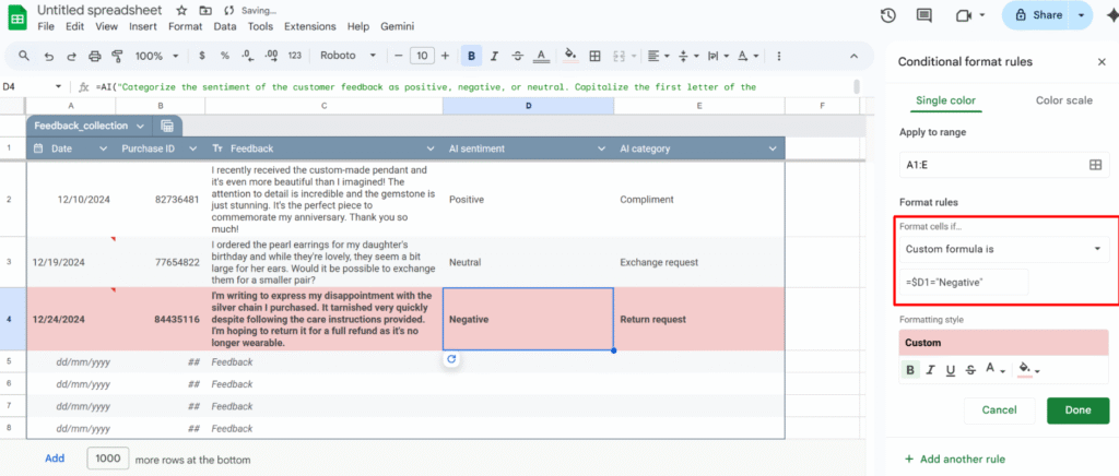
Highlight an entire row based on a single cell
One of the most common questions: “I want the whole row to change color when the status is ‘Done’ / the date is today / the checkbox is ticked.”
Example: highlight every review row where column D is "Negative".
1 – Open Conditional format rules (Format > Conditional formatting)
2 – Select the range you want to format, e.g. A1:E1000.
3 – Under “Format rules”, choose “Custom formula is“
4 – Insert the formula:
=$D1="Negative"
5 – Choose your formatting style and click Done.
Because the range starts at row 1, the formula uses =$D1. If your range starts at row 2 (for example, you skipped the header row), you’d use:
=$D2="Negative"
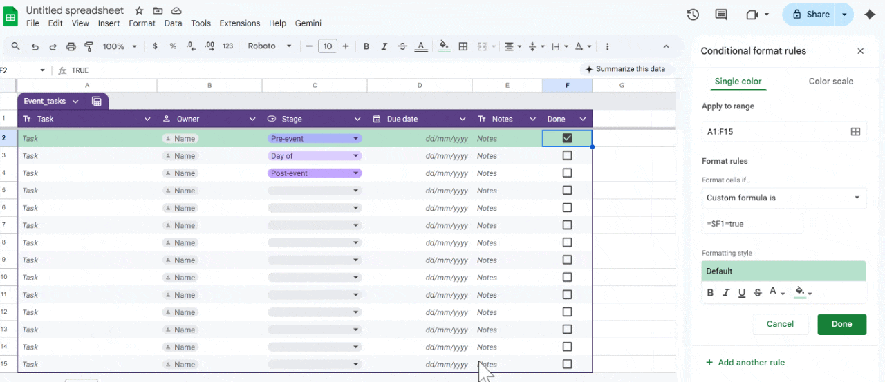
Use checkboxes to drive your formatting and logic
You can use checkboxes as a simple “on/off” switch to control formatting.
Example: highlight the entire row when the checkbox in column F is checked.
Format → Conditional formatting → Custom formula is:
Insert checkboxes in A1:F1000
Select the range to format, e.g. A1:F1000.
=$F1=true
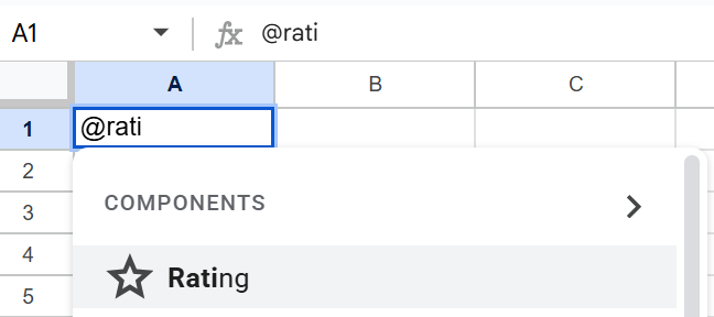
Turn ratings into a quick dropdown (@rating)
If you want fast feedback in a sheet (for tasks, clients, content, etc.), convert a column into a simple rating system.
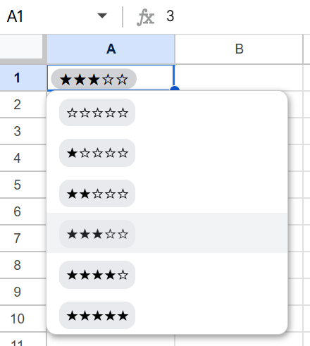
With the Rating smart chip (@rating):
In a cell, type @rating and insert the Rating component.
It creates a small star-based rating widget you can click to set the score.
You now have:
A consistent rating scale across your sheet.
An easy way to scan what’s high/low rated at a glance.
A clean input that still behaves like a value you can reference in formulas or filters.
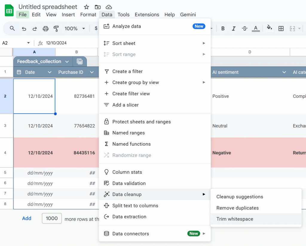
Use Data cleanup
Imported data is messy: extra spaces, duplicates, weird values. Google added built-in cleanup tools that are massively underused.
Cleanup suggestions: A sidebar proposes actions: remove duplicates, fix inconsistent capitalization, etc.
Remove duplicates: You choose the columns to check; Sheets shows how many duplicates it found and removes them.
Trim whitespace: This fixes issues where "ABC" and "ABC " look the same but don’t match in formulas.
Run these before you start building formulas. It saves a lot of debugging time later.
Stop dragging formulas: use ARRAYFORMULA
Common spreadsheet horror story: “My new rows don’t have the formula”, or “someone overwrote a formula with a value”.
ARRAYFORMULAlets you write the formula once and apply it to the whole column.
Example: instead of this in E2:
=B2*C2
and dragging it down, use:
=ARRAYFORMULA(
  IF(
    B2:B="",
    ,
    B2:B * C2:C
  )
)
This:
Applies the multiplication to every row where column B is not empty.
Automatically covers new rows as you add data.
Reduces the risk of someone “breaking” a single cell formula in the middle of your column.
Split CSV-style data into columns (without formulas)
If you’ve ever:
Pasted CSV data into column A,
Used =SPLIT() everywhere,
Then deleted column A manually…
You don’t have to.
Use Data → Split text to columns:
Paste the raw data into one column.
Select that column.
Go to Data → Split text to columns.
Choose the separator (comma, semicolon, space, custom, etc.).
Sheets automatically splits your data into multiple columns without formulas.
Use QUERY instead of copy-pasting filtered tables
Instead of manually filtering and copy-pasting, use QUERY and FILTER to build live views of your data.
Example: from a master task sheet (Sheet4!A1:E), create a separate view with only “To Do” tasks assigned to the person in G2:
=QUERY(
  Sheet4!A1:E,
  "select A, B, C, D, E
   where C = 'To Do'
   and D = '" & G2 & "'
   order by A",
  1
)
Whenever the main sheet is updated, this view updates automatically, no manual copy-paste needed.
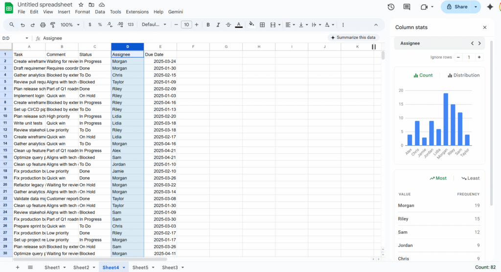
Use column stats to extract quickly key info
If you need a quick snapshot of what’s inside a column—value distribution, most common entries, min/max, etc.—use Column stats.
Right-click a column header.
Select Column stats.
You’ll get:
A count of unique values.
Basic stats (for numbers).
A small chart showing frequency by value.
Store phone numbers and IDs as text (so Sheets doesn’t “fix” them)
Sheets tries to be clever with numbers, which is bad news for things like phone numbers and IDs:
Leading zeros get removed.
Long IDs may be turned into scientific notation.
Best practices:
Set the column to Plain text: Format → Number → Plain text.
Enter numbers with a leading apostrophe: '0412 345 678
Do the same for anything that looks numeric but isn’t a real “number”: phone numbers, SKUs, customer IDs, etc.
This prevents silent changes that are hard to detect later.
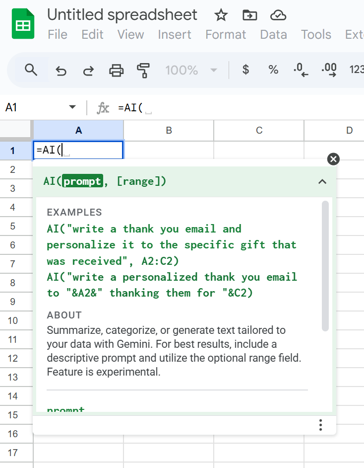
Prompt Gemini directly in your Sheets
Google Sheets now has a native AI function (often exposed as =AI() or =GEMINI(), depending on your Workspace rollout) that lets you talk directly to Google’s Gemini model from a cell.
Instead of nesting complex formulas, you can write natural-language prompts like:
=AI("Summarize this text in 3 bullet points:", A2)
You can use it to:
Summarize long text.
Classify or tag entries.
Extract key information from a sentence.
Generate content (subject lines, slogans, short paragraphs).
Because the prompt and the reference (like A2) live right in the formula, you can apply AI logic across a whole column just like any other function—without touching Apps Script or external tools.
If anything’s missing from this list, tell me! I’d love to hear your favourite Sheets tips and ideas.
Faster dashboards, cleaner code, and a rendering engine powered by the Sheets API.
Google Sheets is fantastic for quick dashboards, tracking tools, and prototypes. And with Apps Script, you can make them dynamic, automated, and even smarter.
But the moment you start building something real, a complex layout, a styled dashboard, a multi-section report, the Apps Script code quickly turns into:
messy
repetitive
slow
painful to maintain
Setting backgrounds, borders, number formats, writing values… everything requires individual calls, and your script balloon quickly.
To make this easier, you usually have two options:
Inject data into an existing template
Or…using RenderSheet
RenderSheet is a tiny, component-based renderer for Google Sheets, inspired by React’s architecture and built entirely in Apps Script. Let’s explore how it works.!
Introducing RenderSheet
RenderSheet is a lightweight, React-inspired renderer for Google Sheets.
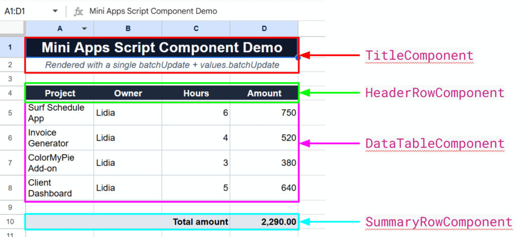
Instead of scattering .setValue(), .setBackground(), .setFontWeight(), etc. everywhere in your script, you write components:
<Title />
<HeaderRow />
<DataTable />
<SummaryRow />
<StatusPill />, etc.
Each component knows how to render itself. Your spreadsheet becomes a clean composition of reusable blocks, just like a frontend UI.
Why a “React-like” approach?
React works because it forces you to think in components:
a Header component
a Table component
a Summary component
a StatusPill component
Each component knows how to render itself, and the app becomes a composition of smaller reusable pieces.I wanted the exact same thing, but for spreadsheets.
With RenderSheet, instead of writing:
sheet.getRange("A1").setValue("Hello");
sheet.getRange("A1").setBackground("#000");
sheet.getRange("A1").setFontWeight("bold");
// and so on...
No direct API calls. No multiple setValue() calls. Just a clean render() method.
The Core Idea: One Render = Two Sheets API Calls
To achieve this “single render” effect, we simply divide to conquer:
one API call for injecting the data
and another for applying all the styling
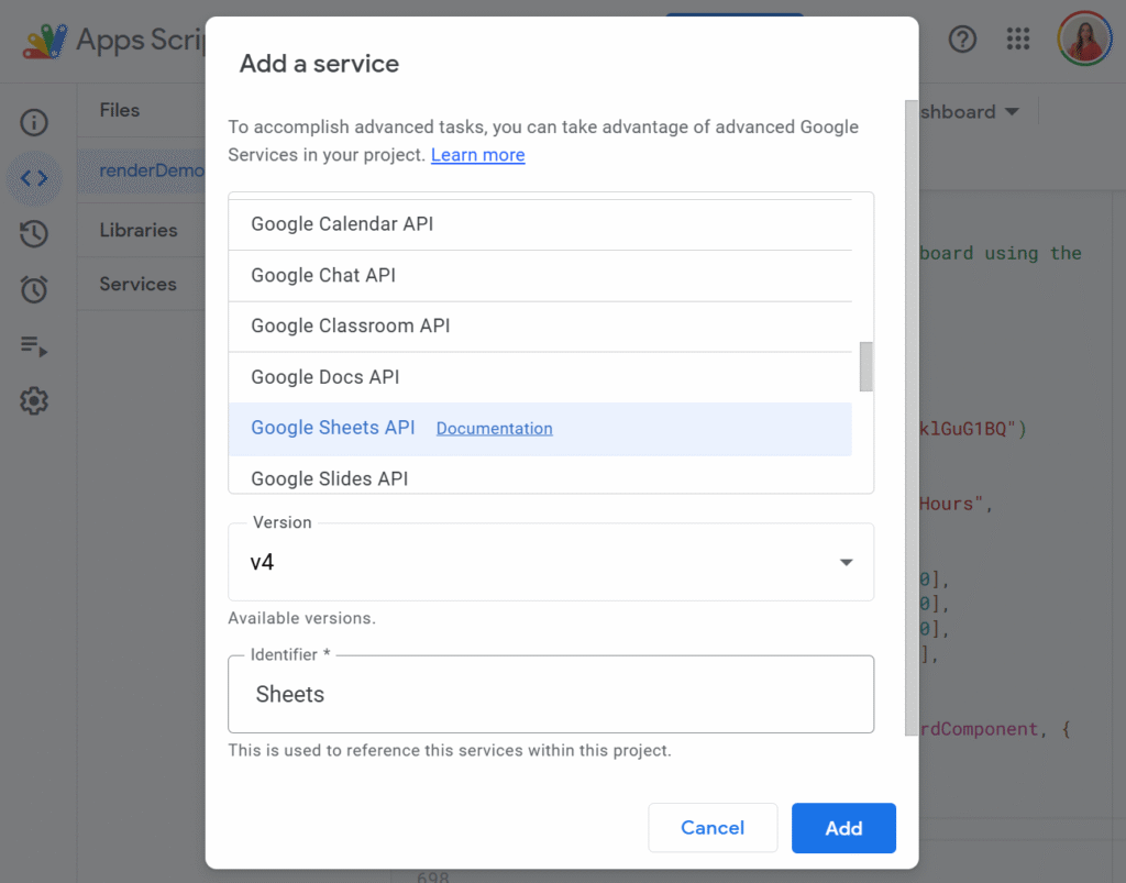
Before we can make the magic happen, we need to enable the Advanced Google Sheets API in our Apps Script project. This unlocks the batchUpdate method, the real engine behind RenderSheet.
To do so, just click the little + button on the left side panel, in front of Services, and select Google Sheets API:
This gives you access to the batchUpdate method, the real engine behind RenderSheet.
Now let’s look at the core mechanism.
The SheetContext (the Render Engine)
SheetContextis the core of RenderSheet. It collects all writes and formatting instructions and applies them in two API calls, using easy functions such as:
all data writes (writeRange)
all formatting instructions (setBackground, setTextFormat, setAlignment…)
But here’s the key:
None of these functions execute anything immediately. They only describe what the component wants to render.
The actual rendering only happens at the end, through two API calls.
You can think of SheetContext as your “toolbox”, and feel free to extend it with your own helpers.
Even though the initial setup is a bit more structured, the final result:
renders in 1 second
stays perfectly maintainable
allows components to be reused in any dashboard
Exactly the power of React, but in Google Sheets.
Final Thoughts
RenderSheet brings structure, speed, and clarity to Google Sheets development. If you’re tired of repetitive formatting code or want to build Sheets dashboards the same way you build UIs, this pattern completely changes the experience.
Let me know what you think, and feel free to contribute!
Even if I’m a real advocate of Apps Script, I’m also very aware of its limits when it comes to performance.
When a script keeps fetching the same API data or repeatedly processes large spreadsheets, things slow down fast. Each execution feels heavier than the previous one, and you end up wasting both user time and valuable API quota. Caching solves this problem by avoiding unnecessary work.
In this article, we’ll walk through what a cache actually is, how the Cache Service works in Apps Script, and the situations where it makes a real difference.
What’s a Cache?
A cache is simply a temporary storage area that keeps data ready to use. Instead of computing something again or fetching it every time, you store the result once, and reuse it for a short period.
For example, imagine calling an external API that takes half a second to respond. If you cache the result for five minutes, the next calls come back instantly. The data isn’t stored forever, just long enough to avoid waste.
This principle is everywhere in tech: browsers, databases, CDNs… and Google Apps Script has its own version too.
What Is Cache Service in Apps Script?
The Cache Service in Google Apps Script gives you a small, fast place to store temporary data. It comes in three “scopes” depending on your use case:
Data shared across all users of your script (getScriptCache)
Data specific to the current user (getUserCache)
Data linked to a particular document (getDocumentCache)
It only stores strings, which means that objects need to beserialized (JSON.stringify). The storage is also limited in size and duration: up to 100 KB per key, and a lifetime of up to 6 hours.
It’s not meant to replace a database or a sheet, it’s meant to speed up your script by avoiding repetitive or heavy work.
When Should You Use It?
Speeding up repeated API calls
If your script fetches data from GitLab, Xero, or any third-party API, calling that API every time is unnecessary. The Cache Service is ideal for storing the latest response for a few minutes. Your script becomes faster, and you avoid hitting rate limits.
Avoiding expensive spreadsheet reads
Large spreadsheets can be slow to read. If you always transform the same data (for example: building a dropdown list, preparing a JSON structure, or filtering thousands of rows), caching the processed result saves a lot of execution time.
Making HTMLService UIs feel instant
Sidebars and web apps built with HTMLService often reload data each time they open. If that data doesn’t need to be fresh every second, keeping it in cache makes the UI load instantly and improves the user experience noticeably.
Storing lightweight temporary state
For short-lived information—like a user’s last selected filter or a temporary calculation—Cache Service is much faster than PropertiesService, and avoids writing into Sheets unnecessarily.
A Simple Way to Use Cache Service
You can create a small helper function that retrieves data from the cache when available, or stores it if missing:
/**
 * Returns cached data or stores a fresh value if missing.
 * @param {string} key
 * @param {Function} computeFn Function that generates fresh data
 * @param {number} ttlSeconds Cache duration in seconds
 * @return {*} Cached or fresh data
 */
function getCached(key, computeFn, ttlSeconds = 300) {
  const cache = CacheService.getScriptCache();
  const cached = cache.get(key);
  if (cached) return JSON.parse(cached);

  const result = computeFn();
  cache.put(key, JSON.stringify(result), ttlSeconds);
  return result;
}
And use it like this:
function getProjects() {
  return getCached('gitlab_projects', () => {
    const res = UrlFetchApp.fetch('https://api.example.com/projects');
    return JSON.parse(res.getContentText());
  });
}
This approach is enough to dramatically speed up most Apps Script projects.
Final Thoughts
The Cache Service is small, simple, but incredibly effective if used well. It won’t store long-term data and it won’t replace a database, but for improving performance and reducing unnecessary work, it’s one of the easiest optimizations you can add to an Apps Script project.
If you want, I can help you write a second article with more advanced techniques: cache invalidation, dynamic keys, TTL strategies, and UI refresh patterns.
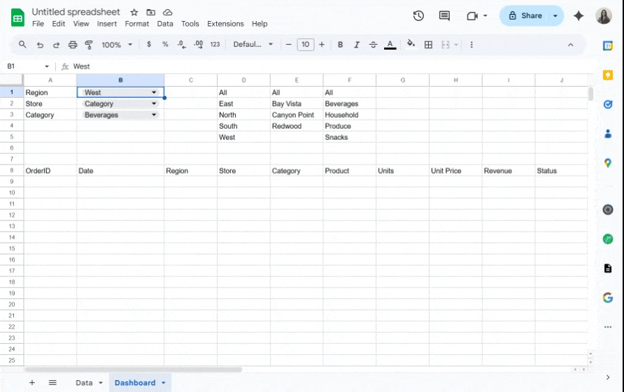
Dashboards feel magical when they react instantly to a selection, no scripts, no reloads, just smooth changes as you click a dropdown.
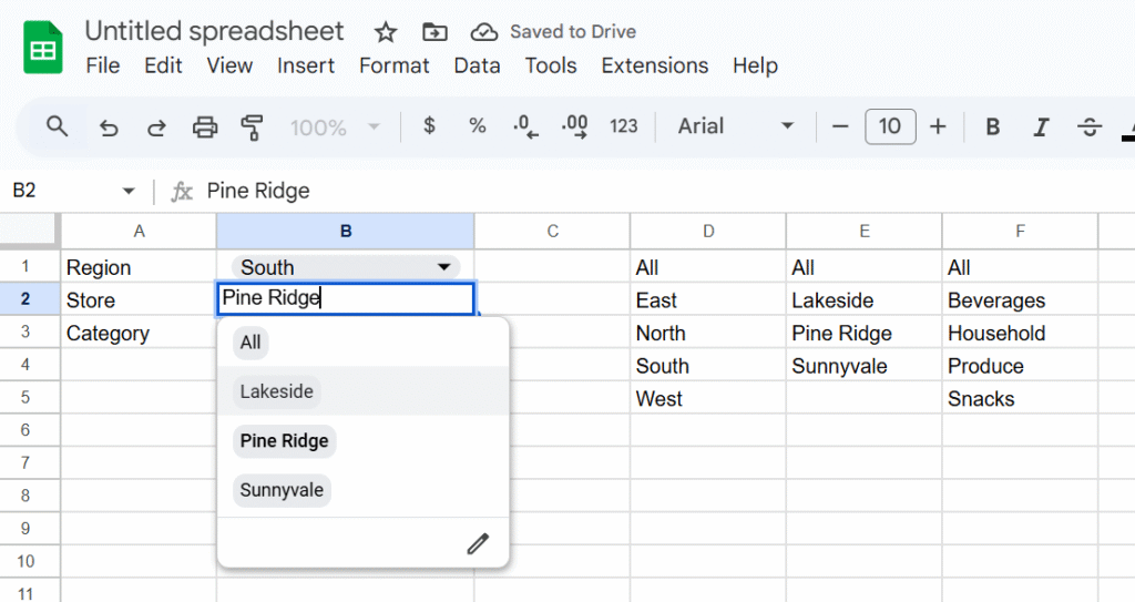
In this tutorial, we will build exactly that in Google Sheets: pick a Region, optionally refine by Store and Category, and watch your results table update in real time. We’ll use built-in tools, Data validation for dropdowns and QUERY for the live results, so it’s fast, maintainable, and friendly for collaborators.
In this example, we’ll use a sales dataset and create dropdowns for Region, Store, and Category, but you can easily adapt the approach to your own data and fields.
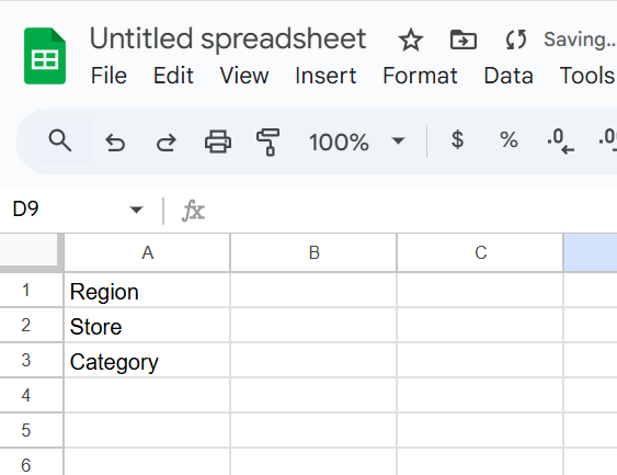
Step 1 – Add control labels
Let’s create a sheet, named Dashbaord, and add
A1:Region
A2:Store (dependent on Region)
A3:Category
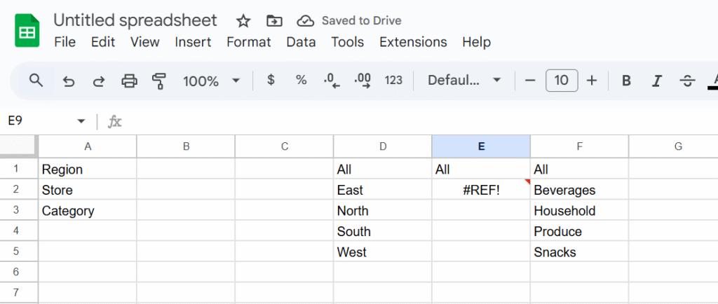
Step 2 – Build dynamic lists (helper formulas)
In column D, we will create a dynamic list of region with the following formula (insert the formula in D1):
Google Sheets is amazing, until it isn’t. As your spreadsheets grow with formulas, collaborators, and live data, they can get painfully slow. Here are all the tricks I’ve found to help my clients get better performances.
Why Google Sheets Get Slow
Too many formulas, especially volatile ones (NOW(), TODAY(), RAND())
Large datasets (thousands of rows/columns)
Repeated or redundant calculations
Overuse of heavy formulas or IMPORTRANGE, ARRAYFORMULA, QUERY…
Dozens of collaborators editing simultaneously
Conditional formatting or custom functions on big ranges
Quick Fixes to Speed Things Up
✔️ Tidy Up Your Formulas
Start by removing or replacing volatile functions like NOW() or RAND() with static values when you don’t need them to update constantly. Use helper columns to calculate something once and reference that instead of repeating logic across rows.
Use fixed ranges (A2:A1000) instead of full-column references. Every formula referencing A:A makes Google Sheets look at all 50,000+ possible rows, even if you’re only using 1,000.
✔️ Lighten the Load
Think of your sheet as a backpack: if it’s stuffed with years of unused data and unnecessary features, it’ll be slow to move. Delete unused rows and columns. Archive old data to separate files. Keep the main spreadsheet focused on what matters now.
✔️ Be Visual, Not Flashy
Conditional formatting, while beautiful, is a silent performance killer. Use it selectively and avoid applying rules to entire columns or rows. Likewise, go easy on charts and embedded images. Move your dashboards to a separate file if needed.
Apps Script and Heavy-Duty Sheets
When dealing with large spreadsheets, your scripting strategy matters. Google Apps Script offers two main interfaces: SpreadsheetApp and the advanced Sheets API. While SpreadsheetApp is easier to use, it becomes painfully slow with big datasets because it handles operations cell by cell.
Instead, for serious performance, we lean heavily on the Sheets API and its batchUpdate method. This allows us to push changes to many cells at once, minimizing round trips and drastically speeding up execution.
Here’s a simple example that injects data into a large range using the Sheets API, not SpreadsheetApp:
// Example of data
const data = [{
  "range": "A35",
  "values": [["TEST"]]
}];

/**
 * Write to multiple, disjoint data ranges.
 * @param {string} spreadsheetId The spreadsheet ID to write to.
 * @see https://developers.google.com/sheets/api/reference/rest/v4/spreadsheets.values/batchUpdate
 */
function writeToMultipleRanges(spreadsheetId, data, sheetName) {

  let ssGetUrl = `https://sheets.googleapis.com/v4/spreadsheets/${spreadsheetId}`
  let options = {
    muteHttpExceptions: false,
    contentType: 'application/json',
    method: 'get',
    headers: { Authorization: 'Bearer ' + ScriptApp.getOAuthToken() }
  };
  let ssGetresponse = JSON.parse(UrlFetchApp.fetch(ssGetUrl, options));
  let sheets = ssGetresponse.sheets;
  let rowCount = 0;
  let sheetId = 0;
  sheets.forEach(sheet => {
    if (sheet.properties.title == sheetName) {
      rowCount = sheet.properties.gridProperties.rowCount
      sheetId = sheet.properties.sheetId;
    }
  });

  let num = parseInt(String(data[0]["range"]).split("!")[1].replace(/[^0-9]/g, ''));
  if (rowCount < num) {
    let diff = num - rowCount;
    let resource = {
      "requests": [
        {
          "appendDimension": {
            "length": diff,
            "dimension": "ROWS",
            "sheetId": sheetId
          }
        }
      ]
    };
    let ssBatchUpdateUrl = `https://sheets.googleapis.com/v4/spreadsheets/${spreadsheetId}:batchUpdate`
    let options = {
      muteHttpExceptions: true,
      contentType: 'application/json',
      method: 'post',
      payload: JSON.stringify(resource),
      headers: { Authorization: 'Bearer ' + ScriptApp.getOAuthToken() }
    };
    let response = JSON.parse(UrlFetchApp.fetch(ssBatchUpdateUrl, options));
  }

  const request = {
    'valueInputOption': 'USER_ENTERED',
    'data': data
  };

  try {
    const response = Sheets.Spreadsheets.Values.batchUpdate(request, spreadsheetId);
    if (response) {
      return;
    }
    console.log('response null');
  } catch (e) {
    console.log('Failed with error %s', e.message);
  }
}

/**
 * Converts a row and column index to A1 notation (e.g., 3, 5 → "E3").
 *
 * @param {number} rowIndex - The 1-based row index.
 * @param {number} colIndex - The 1-based column index.
 * @returns {string} The A1 notation corresponding to the given indices.
 */
function getA1Notation(rowIndex, colIndex) {
  if (rowIndex < 1 || colIndex < 1) {
    throw new Error("Both rowIndex and colIndex must be greater than or equal to 1.");
  }
  let columnLabel = "";
  let col = colIndex;
  while (col > 0) {
    const remainder = (col - 1) % 26;
    columnLabel = String.fromCharCode(65 + remainder) + columnLabel;
    col = Math.floor((col - 1) / 26);
  }
  return columnLabel + rowIndex;
}
Freeze Formulas
Often, you only need a formula to calculate once, not every time the sheet updates.
Instead of leaving it active and recalculating endlessly, you can use Apps Script to compute the values once and then lock them in as static data.
The script below is designed for that: it keeps the original formulas in the second row (as a reference and for future recalculations), then copies those formulas down the column, computes all results, and finally replaces everything below the second row with raw values. The result? A faster sheet that still preserves its logic blueprint in row two.
/**
 *
 */
function Main_Update_Formula_Data(ssId, sheet) {

  // Get formulas in first row
  const formulas = sheet.getRange(2, 1, 1, sheet.getLastColumn()).getFormulas()[0];

  // Get last row index
  const lastRowIndex = sheet.getLastRow();

  // Prepare ranges to treat
  const ranges = [];

  // Loop through formulas to expand until the end
  for (let i = 0; i < formulas.length; i++) {

    if (formulas[i] != ""
      && !String(formulas[i]).startsWith("=arrayformula")
      && !String(formulas[i]).startsWith("=ARRAYFORMULA")
      && !String(formulas[i]).startsWith("=ArrayFormula")) {

      const thisRange = {
        startRowIndex: 1,
        endRowIndex: lastRowIndex - 1,
        startColumnIndex: i,
        endColumnIndex: i + 1,
        formulas: [formulas[i]],
      };

      ranges.push(thisRange);
    }
  }

  // Inject and freeze data except first row of formulas
  injectAndFreezeFormulas(ssId, sheet.getSheetId(), sheet.getName(), ranges);
}


/**
 * Injects formulas into multiple ranges, waits for computation, then replaces them with static values.
 * @param {string} spreadsheetId - Spreadsheet ID.
 * @param {number} sheetId - Numeric sheet ID.
 * @param {string} sheetName - Sheet name (for value reads/writes).
 * @param {Array<Object>} ranges - Array of range configs like:
 * @return {void}
 */
function injectAndFreezeFormulas(spreadsheetId, sheetId, sheetName, ranges) {
  // --- Inject formulas via batchUpdate
  const requests = [];
  ranges.forEach(rangeDef => {
    const {
      startRowIndex,
      endRowIndex,
      startColumnIndex,
      endColumnIndex,
      formulas,
    } = rangeDef;

    formulas.forEach((formula, idx) => {
      requests.push({
        repeatCell: {
          range: {
            sheetId,
            startRowIndex,
            endRowIndex,
            startColumnIndex: startColumnIndex + idx,
            endColumnIndex: startColumnIndex + idx + 1,
          },
          cell: {
            userEnteredValue: { formulaValue: formula },
          },
          fields: 'userEnteredValue',
        },
      });
    });
  });

  Sheets.Spreadsheets.batchUpdate({ requests }, spreadsheetId);
  Logger.log(`Formulas injected into ${ranges.length} range(s)`);

  // --- Wait briefly to ensure calculations are done
  Utilities.sleep(1000);

  // --- Read computed values via API (valueRenderOption: UNFORMATTED_VALUE)
  const readRanges = ranges.map(r =>
    `${sheetName}!${columnLetter(r.startColumnIndex + 1)}3:` +
    `${columnLetter(r.endColumnIndex)}${r.endRowIndex + 1}`
  );

  const readResponse = Sheets.Spreadsheets.Values.batchGet(spreadsheetId, {
    ranges: readRanges,
    valueRenderOption: 'UNFORMATTED_VALUE',
  });

  // --- Reinject values (overwrite formulas)
  const writeData = readResponse.valueRanges.map((vr, idx) => ({
    range: readRanges[idx],
    values: vr.values || [],
  }));

  Sheets.Spreadsheets.Values.batchUpdate(
    {
      valueInputOption: 'RAW',
      data: writeData,
    },
    spreadsheetId
  );

  Logger.log(`Formulas replaced by static values in ${writeData.length} range(s)`);
}

/**
 * Helper — Convert a column index (1-based) to A1 notation.
 *
 * @param {number} colIndex - 1-based column index.
 * @return {string}
 */
function columnLetter(colIndex) {
  let letter = '';
  while (colIndex > 0) {
    const remainder = (colIndex - 1) % 26;
    letter = String.fromCharCode(65 + remainder) + letter;
    colIndex = Math.floor((colIndex - 1) / 26);
  }
  return letter;
}
Did you know all of these tricks? If you’ve got a favorite performance tip, clever automation, or formula hack, drop it in the comments! Let’s keep our Sheets smart, fast, and fun to work with.
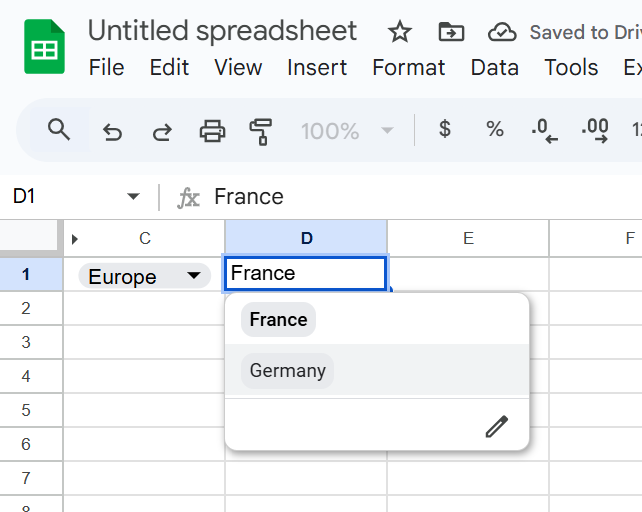
Google Sheets drop-downs are a great way to control inputs and keep your data clean. A classic use case is to have different options for a drop down, depending on what was selecting in another.
That’s where dependent drop-down lists (also called cascading drop-downs) come in. For example:
In Drop-Down 1, you select a Region (Europe, Asia, America).
In Drop-Down 2, you only see the Countries from that region (Europe → France, Germany, Spain).
This guide shows you step by step how to build dependent drop-downs in Google Sheets — without named ranges, using formulas and a simple script for better usability.
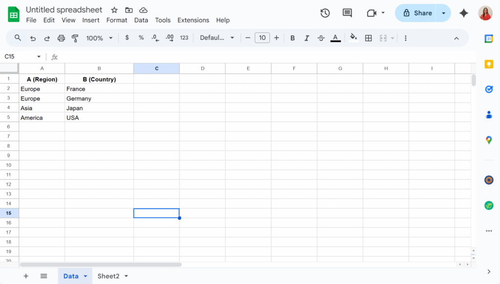
Step 1 – Organize your source data
On a sheet named Data, enter your list in two columns:
Important: Use one row per country (don’t put “France, Germany, Spain” in a single cell).
Step 2 – Create the drop-down lists
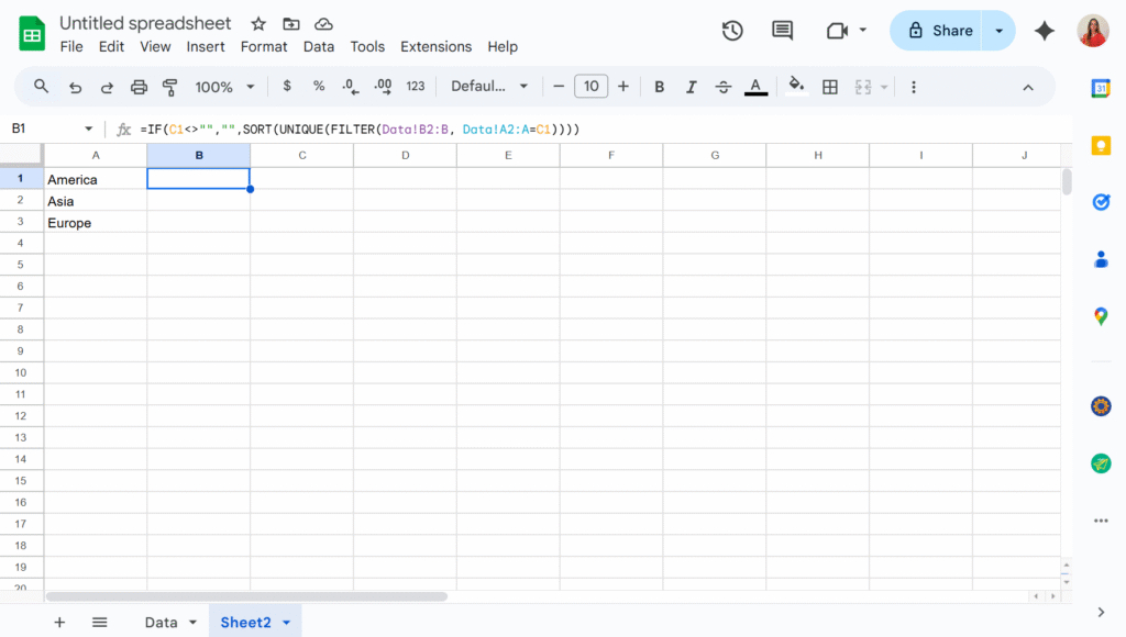
The key is not to link drop-downs directly to your raw lists, but to use formulas that generate the lists dynamically. These formulas can live on the same sheet as your data or on a separate one. In this example, I’ll place them in Sheet2 to keep the Data sheet uncluttered.
In A2, I will add the formula:
=SORT(UNIQUE(FILTER(Data!A2:A, Data!A2:A<>"")))
This way, the first drop-down will display a clean list of countries without any duplicates.
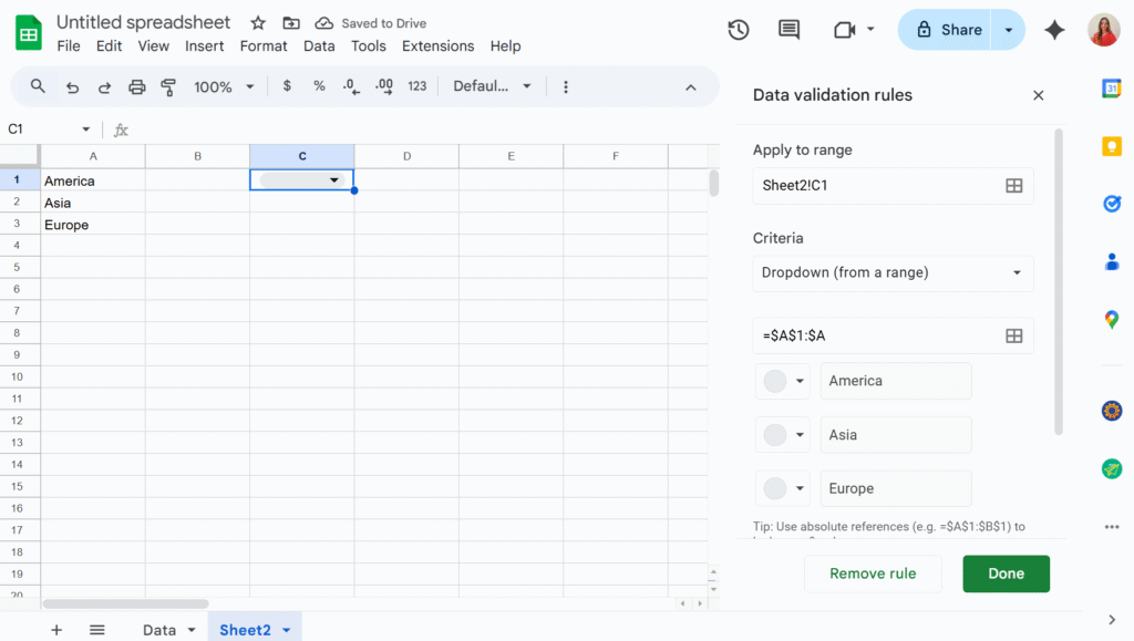
And in B2, assuming the country drop-down will be in C1 :
Now we can simply add two drop-downs in C1 and D1, using the “Dropdown from a range” option in the Data validation menu.
The second drop-down will now display only the values that match the selection from the first drop-down. You can then hide columns A and B to keep your sheet tidy — and voilà!
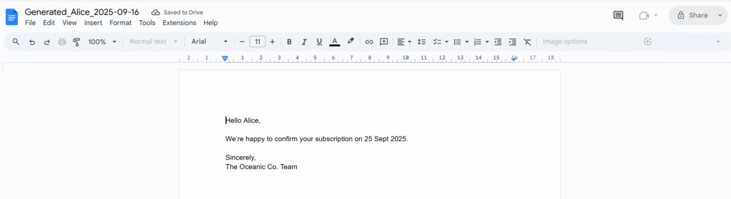
In othe previous article, we learned how to replace placeholders like [name] or [date] inside a Google Doc using Apps Script. We also made sure to keep the original file intact by creating a copy before applying replacements.
That’s great for a single document… but what if you need to create dozens of personalized files? Contracts, certificates, letters, all with different values?
The answer: connect your Google Doc template to a Google Sheet. Each row of your sheet will represent a new document, and the script will:
Create a copy of the template
Replace all placeholders with values from the sheet
Paste the link of the generated file back into the spreadsheet
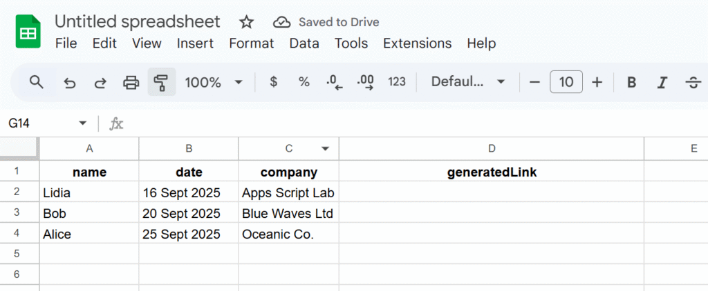
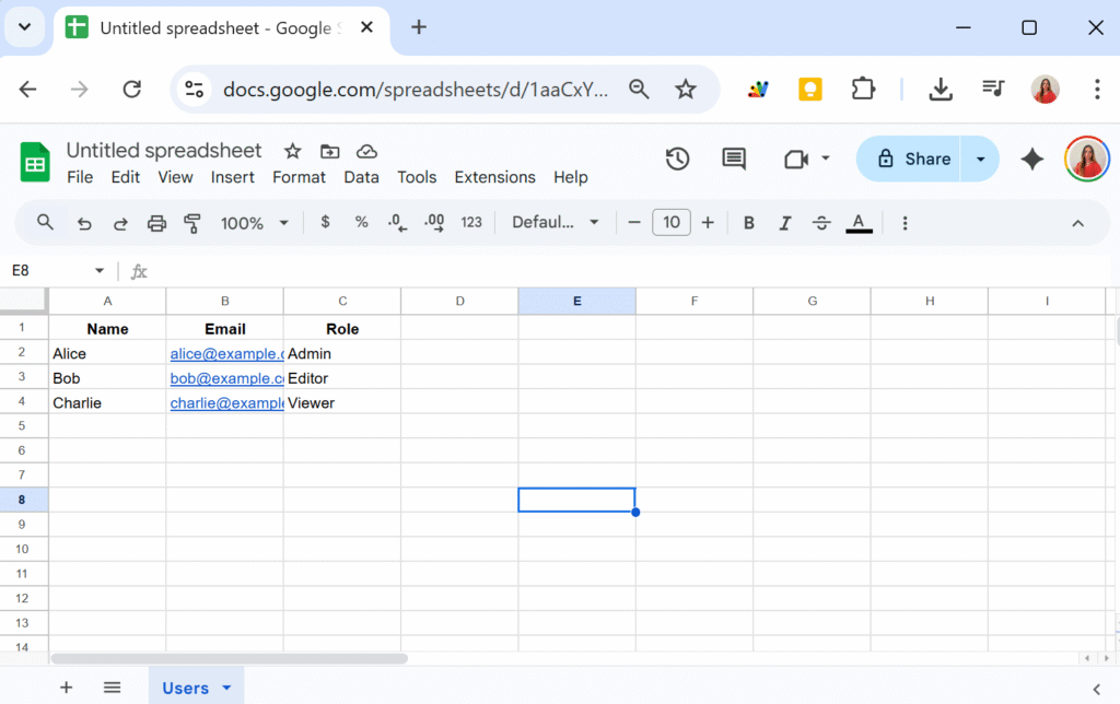
Step 1 – Prepare your Spreadsheet
Create a sheet with the following structure (headers in the first row):
Notice the last column generatedLink, that’s where the script will paste the URL of each generated document.
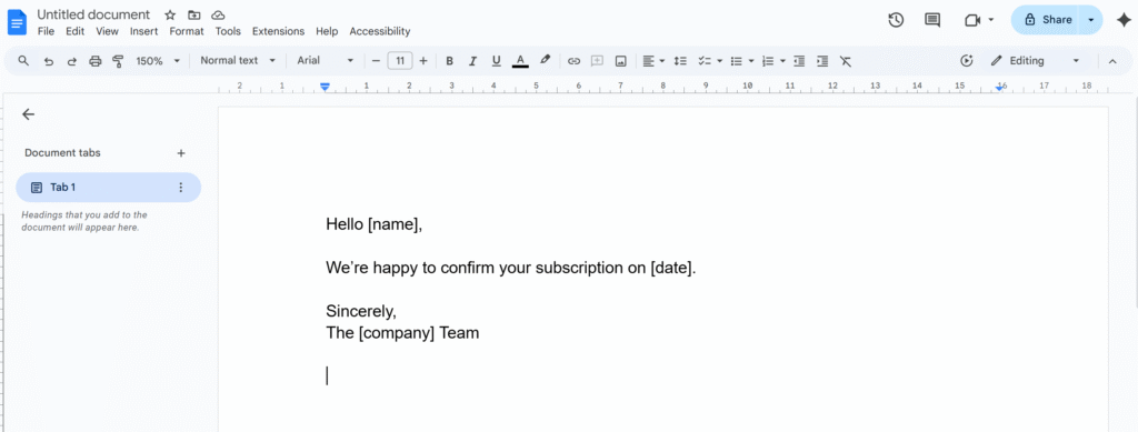
Step 2 – Prepare your Google Doc Template
In your template, write placeholders between brackets:
Step 3 – The Script
This time the script will be bounded to our Google Sheets.
Open the Apps Script editor from your Spreadsheet (Extensions → Apps Script) and paste:
/**
 * Generate documents from a template Doc,
 * replacing placeholders with data from the sheet,
 * and storing links back in the sheet.
 */
function generateDocsFromSheet() {
  // IDs
  const TEMPLATE_ID = 'YOUR_TEMPLATE_DOC_ID_HERE';
  const FOLDER_ID = 'YOUR_TARGET_FOLDER_ID_HERE';

  const ss = SpreadsheetApp.getActiveSpreadsheet();
  const sheet = ss.getActiveSheet();
  const data = sheet.getDataRange().getValues();
  const headers = data[0];

  // Loop through each row (skip headers)
  for (let i = 1; i < data.length; i++) {
    const row = data[i];

    // Skip if doc already generated
    if (row[headers.indexOf('generatedLink')]) continue;

    // Build replacements
    const replacements = {};
    headers.forEach((h, idx) => {
      if (h !== 'generatedLink') {
        replacements[`\\[.*${h}.*\\]`] = row[idx];
      }
    });

    // Make copy of template
    const templateFile = DriveApp.getFileById(TEMPLATE_ID);
    const copyFile = templateFile.makeCopy(
      `Generated_${row[0]}_${new Date().toISOString().slice(0,10)}`,
      DriveApp.getFolderById(FOLDER_ID)
    );

    // Open and replace placeholders
    const doc = DocumentApp.openById(copyFile.getId());
    const body = doc.getBody();
    for (let tag in replacements) {
      body.replaceText(tag, replacements[tag]);
    }
    doc.saveAndClose();

    // Save link back into sheet
    sheet.getRange(i+1, headers.indexOf('generatedLink')+1)
      .setValue(copyFile.getUrl());
  }
}
Step 4 – Run the Script
Replace YOUR_TEMPLATE_DOC_ID_HERE with your template’s Doc ID
Replace YOUR_TARGET_FOLDER_ID_HERE with the ID of the folder where generated docs should be stored
Run the script → authorize it → watch your documents appear!
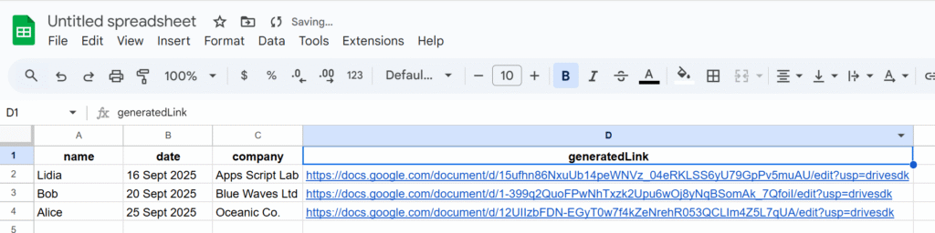
Each row in your sheet now produces a new Google Doc, and the link is written back automatically:
Wrap Up
With just a few lines of code, you’ve upgraded your document automation:
One Google Doc becomes a reusable template
One Google Sheet becomes a data source
Each row produces a personalized document with its link logged back
This setup is basically a DIY mail-merge for Docs
In the next article, we’ll explore how to send those generated documents automatically by email, turning your workflow into a fully automated system.
That format is fine for small scripts, but it quickly becomes messy. You end up with unreadable code like:
const data = sheet.getDataRange().getValues();
for (let i = 1; i < data.length; i++) {
  const name = data[i][0];
  const email = data[i][1];
  const role = data[i][2];
  // ...
}
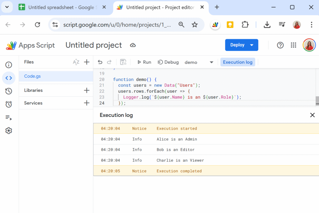
Hard to read. Easy to break. And if someone reorders the spreadsheet columns, your code will suddenly pull the wrong data.
A Cleaner Way: Convert to Array of Objects
Instead of juggling indexes, let’s wrap the data in a class that automatically maps each row into an object , using the first row of the sheet as headers.
class Data {
  constructor(sheetName) {
    this.spreadsheet = SpreadsheetApp.getActiveSpreadsheet();
    this.sheetName = sheetName;
    this.sheet = this.spreadsheet.getSheetByName(this.sheetName);

    if (!this.sheet) throw `Sheet ${this.sheetName} not found.`;

    const data = this.sheet.getDataRange().getValues();
    this.headers = data.shift();
    this.rows = data.map(row =>
      row.reduce((record, value, i) => {
        record[this.headers[i]] = value;
        return record;
      }, {})
    );
  }
}
Now, when we create a new Data instance:
function demo() {
  const users = new Data("Users");
  Logger.log(users.rows);
}
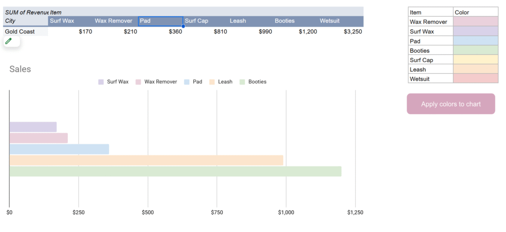
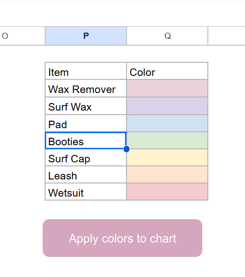
Have you ever noticed that chart colors in Google Sheets sometimes shuffle around when your data changes? This usually happens when you build a chart on top of a pivot table. If one of the series (like a product or category) isn’t present in the filtered data, Google Sheets automatically re-assigns colors.
The result: one week “Surf Wax” is blue, the next week it’s orange, and your report suddenly looks inconsistent. Not great if you’re sending charts to clients or managers who expect a clean, consistent palette.
In this tutorial, we’ll fix the problem once and for all by locking chart colors using the Google Sheets API from Apps Script.
Why the colors shuffle
Charts in Google Sheets don’t store colors per label by default, they store them per series position. So if your chart shows [Surf Wax, Leash, Wetsuit] this week, those get assigned colors 0, 1, 2. But if next week [Pad] is missing, everything shifts left and the colors move with them.
That’s why you see colors “jump” around when some categories are empty.
The fix: define your own color map
The solution is to create a color map table in your sheet that tells Apps Script what color each item should always use.
Example in range P2:Q:
The trick is that we don’t actually use the text in the “Color” column, we use the cell background color. This makes it easy to set and change colors visually.
Using the Sheets API to lock colors
The built-in SpreadsheetApp class in Apps Script doesn’t let us fully control chart series. For that, we need the Advanced Sheets Service (a wrapper around the Google Sheets REST API).
To enable it:
In the Apps Script editor, go to Services > Add a service > turn on Google Sheets API v4.
The Apps Script solution
Here’s the script that applies your custom colors to the first chart on the Sales sheet:
/**
 * Apply chart colors from mapping in P2:Q to the first chart in "Sales".
 */
function updateChartColors() {
  const ss = SpreadsheetApp.getActiveSpreadsheet();
  const sheet = ss.getSheetByName("Sales");
  const spreadsheetId = ss.getId();

  // 1. Build color map (Item -> hex from background)
  const mapRange = sheet.getRange("P2:Q");
  const values = mapRange.getValues();
  const bgs = mapRange.getBackgrounds();

  const colorMap = {};
  values.forEach((row, i) => {
    const item = row[0];
    const color = bgs[i][1];
    if (item && color && color !== "#ffffff") {
      colorMap[item] = color;
    }
  });

  // 2. Get chart spec from Sheets API
  const sheetResource = Sheets.Spreadsheets.get(spreadsheetId, {
    ranges: [sheet.getName()],
    fields: "sheets(charts(chartId,spec))"
  }).sheets[0];

  if (!sheetResource.charts) return;
  const chart = sheetResource.charts[0];
  const chartId = chart.chartId;
  const spec = chart.spec;

  // 3. Apply colors by matching series headers with map
  if (spec.basicChart && spec.basicChart.series) {
    spec.basicChart.series.forEach((serie, i) => {
      const src = serie.series?.sourceRange?.sources?.[0];
      if (!src) return;

      // Get header label (like "Surf Wax", "Leash", etc.)
      const header = sheet.getRange(
        src.startRowIndex + 1,
        src.startColumnIndex + 1
      ).getValue();

      if (colorMap[header]) {
        spec.basicChart.series[i].colorStyle = {
          rgbColor: hexToRgbObj(colorMap[header])
        };
      }
    });
  }

  // 4. Push update back into the chart
  Sheets.Spreadsheets.batchUpdate(
    {
      requests: [
        {
          updateChartSpec: {
            chartId,
            spec
          }
        }
      ]
    },
    spreadsheetId
  );
}

/**
 * Convert #RRGGBB hex to Sheets API {red, green, blue}.
 */
function hexToRgbObj(hex) {
  const bigint = parseInt(hex.slice(1), 16);
  return {
    red: ((bigint >> 16) & 255) / 255,
    green: ((bigint >> 8) & 255) / 255,
    blue: (bigint & 255) / 255
  };
}
How it works
Read the color map from P2:Q using the cell background color.
Fetch the chart spec from the Sheets API.
For each series, look up the header label from the pivot table (like “Wax Remover”).
If it exists in the map, apply the mapped color using colorStyle: { rgbColor: … }.
Push the modified spec back to the chart with updateChartSpec.
The result: your chart always uses the same colors, no matter which categories are present.
Wrapping up
With this approach, you’ll never have to worry about Google Sheets “helpfully” reshuffling your chart colors again. Once you set your palette in the sheet, a single click on a button can re-apply it to your chart. And because it uses the Sheets API directly, the colors are actually saved in the chart definition itself.
That means your reports stay consistent, your managers stop asking “why is Surf Wax orange this week?”, and your charts look clean and professional every time.
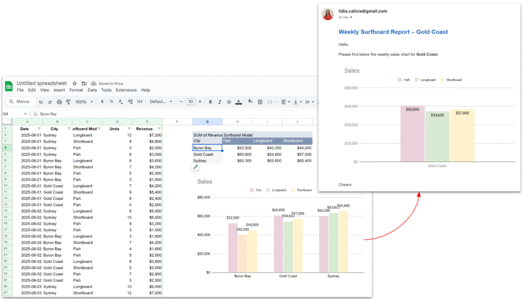
In many reporting workflows, it’s helpful to send reports straight from a spreadsheet, complete with a chart inside the email. Imagine you’re running a surf shop with branches in different cities. Every week, the managers are waiting for their sales report: you filter the data for Sydney, copy the chart, paste it into an email, then repeat the same steps for Byron Bay and the Gold Coast. Before long, it feels like you’re stuck doing the same routine again and again.
Instead of preparing these reports by hand, the whole process can be automated. With a little help from Google Apps Script, the spreadsheet can filter the data for each city, update the chart, and send the report by email automatically.
In this tutorial, we will see how to:
Extract a list of unique cities from the sales data.
Apply a pivot filter dynamically for each city.
Capture the chart as an image.
Send a nicely formatted email with the chart embedded directly in the body.
We’ll go through the script function by function.
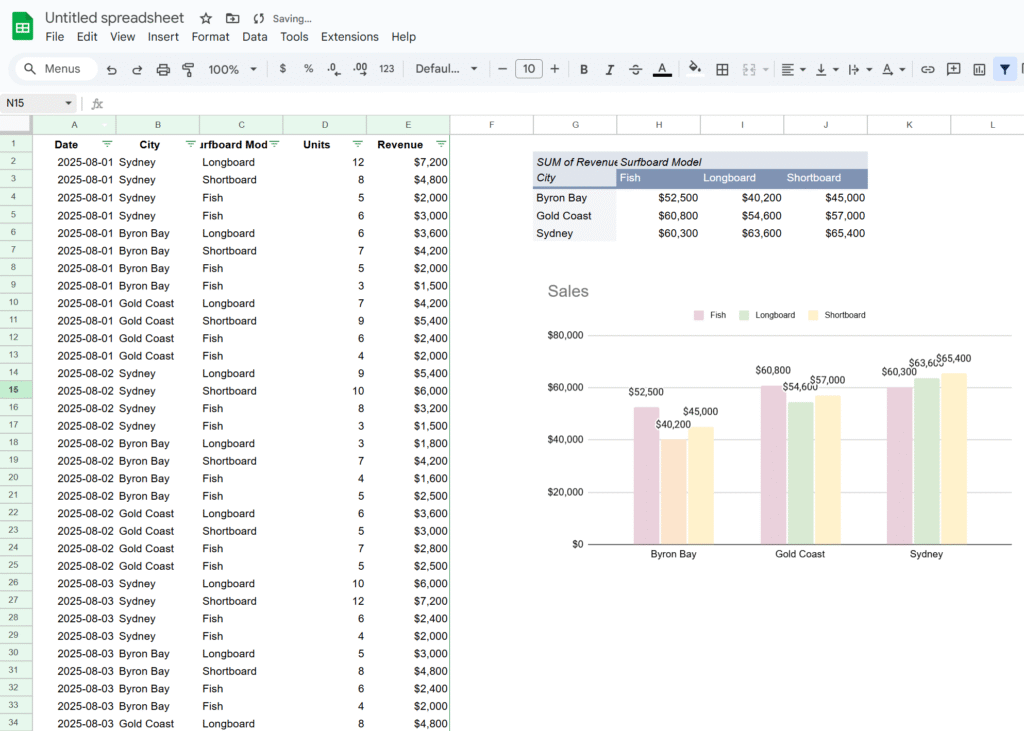
Here’s the Google Sheet we’ll be using in this tutorial, containing a simple dataset along with a pivot table and a chart.
1. Main function – looping through cities
Our entry point is the sendWeeklyReports() function.
function sendWeeklyReports() {
  // Getting sheet and data
  const ss = SpreadsheetApp.getActiveSpreadsheet();
  const salesSheet = ss.getSheetByName("Sales");
  const salesData = salesSheet.getDataRange().getValues();
  const headers = salesData.shift();

  // Extract cities
  const cities = salesData.map(x => x[headers.indexOf("City")]);

  // Get unique list of cities
  const unqiueCities = new Set(cities);

  // Get pivot table
  const pivotTable = salesSheet.getPivotTables()[0];

  // Get chart
  const chart = salesSheet.getCharts()[0];

  unqiueCities.forEach(city => {
    applyPivotFilter(city, pivotTable);
    const chartBlob = getPivotChartAsImage(chart, city);
    sendEmailReport(city, chartBlob);
  });
}
Explanation:
We grab the entire dataset from the Sales sheet.
From the data, we extract all values in the City column and convert them into a Set → this gives us a unique list of cities. This way, if a new city is added in the future (e.g. Melbourne), it’s automatically included.
We grab the pivot table and chart already created in the sheet.
Finally, we loop through each city, apply a filter, generate the chart image, and send the email.
This main function orchestrates the entire workflow.
2. Filtering the Pivot Table
We need to update the pivot table filter so that it only shows results for one city at a time.
function applyPivotFilter(city, pivotTable) {
  // Remove existing filter
  pivotTable.getFilters().forEach(f => f.remove());

  // Create a criteria for the city
  const criteria = SpreadsheetApp.newFilterCriteria().whenTextContains(city);
  pivotTable.addFilter(2, criteria);

  SpreadsheetApp.flush();
}
Explanation:
First, we clear existing filters. This ensures we don’t stack multiple filters and accidentally hide everything.
Then, we create a new filter criteria for the city.
The addFilter(2, criteria) call means “apply this filter on column index 2” (update this index if your “City” column is different).
Finally, we call SpreadsheetApp.flush() to force Sheets to update the pivot table immediately before we grab the chart.
This function makes the pivot behave as if you clicked the filter dropdown manually and selected just one city.
3. Exporting the Chart as an Image
Once the pivot table is filtered, the chart updates automatically. We can then capture it as an image Blob.
function getPivotChartAsImage(chart, city) {
  return chart.getAs("image/png").setName(`Sales_${city}.png`);
}
Explanation:
chart.getAs("image/png") converts the chart object into an image blob.
We rename the file with the city name, which is handy if you want to attach it or archive it.
This blob can be sent in an email, saved to Drive, or inserted into a Slide deck.
4. Sending the Email
Finally, we embed the chart directly in an HTML email body.
<img src="cid:chartImage"> is a placeholder that’s replaced by the inline chart image.
In the sendEmail call, we pass both the HTML body and inlineImages: { chartImage: chartBlob }.
Result → the chart is embedded in the email itself, not just attached.
This makes the report feel polished and professional.
In conclusion, this workflow shows how easy it is to turn a manual reporting routine into a smooth, automated process. By letting Apps Script filter the pivot table, capture the chart, and send it directly inside an email, you get consistent weekly updates without lifting a finger. It’s a small piece of automation that saves time, reduces errors, and keeps your reports looking professional.
In Google Apps Script, execution time matters. With quotas on simultaneous runs and total runtime, long or inconsistent function execution can cause failures or delays. This is especially important when using services like LockService, where you need to define realistic wait times.
This article shows how to track execution time and errors in your functions—helping you stay within limits and optimize performance as your scripts grow.