Here are 10 Google Sheets tips I use in my day-to-day. You might recognise a few of them, but I’m pretty confident you’ll still learn something new!
Highlight an entire row based on a single cell
One of the most common questions: “I want the whole row to change color when the status is ‘Done’ / the date is today / the checkbox is ticked.”
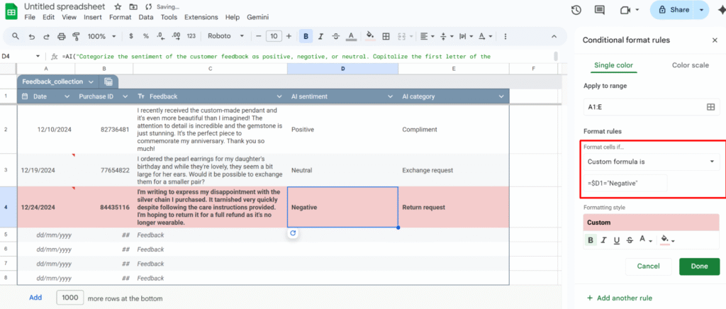
Example: highlight every review row where column D is "Negative".
1 – Open Conditional format rules (Format > Conditional formatting)
2 – Select the range you want to format, e.g. A1:E1000.
3 – Under “Format rules”, choose “Custom formula is“
4 – Insert the formula:
=$D1="Negative"
5 – Choose your formatting style and click Done.
Because the range starts at row 1, the formula uses =$D1. If your range starts at row 2 (for example, you skipped the header row), you’d use:
=$D2="Negative"
Use checkboxes to drive your formatting and logic
You can use checkboxes as a simple “on/off” switch to control formatting.
Example: highlight the entire row when the checkbox in column F is checked.
Format → Conditional formatting → Custom formula is:
Insert checkboxes in A1:F1000
Select the range to format, e.g. A1:F1000.
=$F1=true
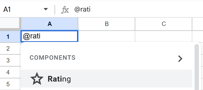
Turn ratings into a quick dropdown (@rating)
If you want fast feedback in a sheet (for tasks, clients, content, etc.), convert a column into a simple rating system.
With the Rating smart chip (@rating):
In a cell, type @rating and insert the Rating component.
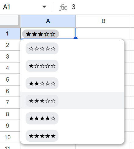
It creates a small star-based rating widget you can click to set the score.
You now have:
A consistent rating scale across your sheet.
An easy way to scan what’s high/low rated at a glance.
A clean input that still behaves like a value you can reference in formulas or filters.
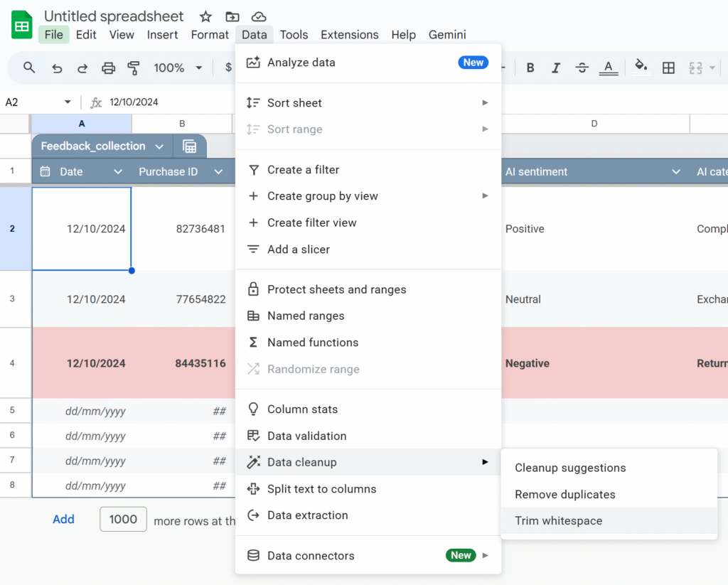
Use Data cleanup
Imported data is messy: extra spaces, duplicates, weird values. Google added built-in cleanup tools that are massively underused.
Cleanup suggestions: A sidebar proposes actions: remove duplicates, fix inconsistent capitalization, etc.
Remove duplicates: You choose the columns to check; Sheets shows how many duplicates it found and removes them.
Trim whitespace: This fixes issues where "ABC" and "ABC " look the same but don’t match in formulas.
Run these before you start building formulas. It saves a lot of debugging time later.
Stop dragging formulas: use ARRAYFORMULA
Common spreadsheet horror story: “My new rows don’t have the formula”, or “someone overwrote a formula with a value”.
ARRAYFORMULAlets you write the formula once and apply it to the whole column.
Example: instead of this in E2:
=B2*C2
and dragging it down, use:
=ARRAYFORMULA(
  IF(
    B2:B="",
    ,
    B2:B * C2:C
  )
)
This:
Applies the multiplication to every row where column B is not empty.
Automatically covers new rows as you add data.
Reduces the risk of someone “breaking” a single cell formula in the middle of your column.
Split CSV-style data into columns (without formulas)
If you’ve ever:
Pasted CSV data into column A,
Used =SPLIT() everywhere,
Then deleted column A manually…
You don’t have to.
Use Data → Split text to columns:
Paste the raw data into one column.
Select that column.
Go to Data → Split text to columns.
Choose the separator (comma, semicolon, space, custom, etc.).
Sheets automatically splits your data into multiple columns without formulas.
Use QUERY instead of copy-pasting filtered tables
Instead of manually filtering and copy-pasting, use QUERY and FILTER to build live views of your data.
Example: from a master task sheet (Sheet4!A1:E), create a separate view with only “To Do” tasks assigned to the person in G2:
=QUERY(
  Sheet4!A1:E,
  "select A, B, C, D, E
   where C = 'To Do'
   and D = '" & G2 & "'
   order by A",
  1
)
Whenever the main sheet is updated, this view updates automatically, no manual copy-paste needed.
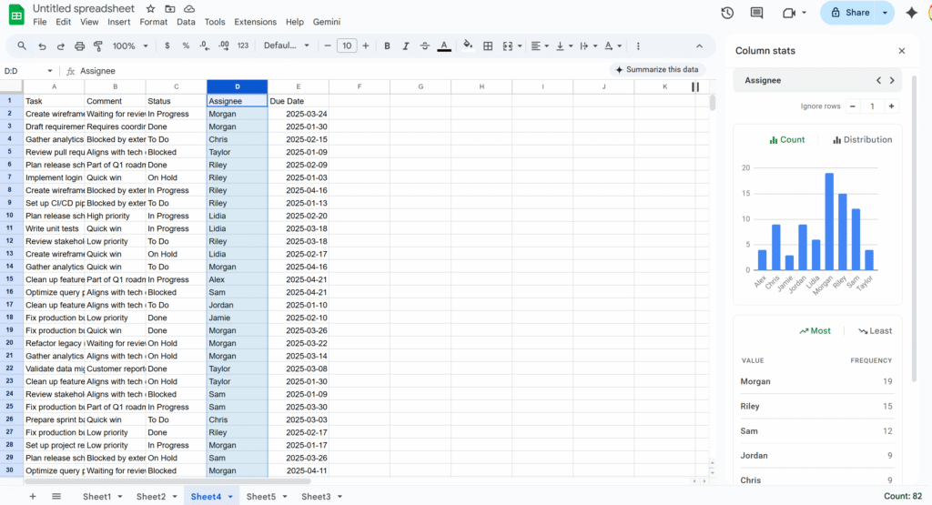
Use column stats to extract quickly key info
If you need a quick snapshot of what’s inside a column—value distribution, most common entries, min/max, etc.—use Column stats.
Right-click a column header.
Select Column stats.
You’ll get:
A count of unique values.
Basic stats (for numbers).
A small chart showing frequency by value.
Store phone numbers and IDs as text (so Sheets doesn’t “fix” them)
Sheets tries to be clever with numbers, which is bad news for things like phone numbers and IDs:
Leading zeros get removed.
Long IDs may be turned into scientific notation.
Best practices:
Set the column to Plain text: Format → Number → Plain text.
Enter numbers with a leading apostrophe: '0412 345 678
Do the same for anything that looks numeric but isn’t a real “number”: phone numbers, SKUs, customer IDs, etc.
This prevents silent changes that are hard to detect later.
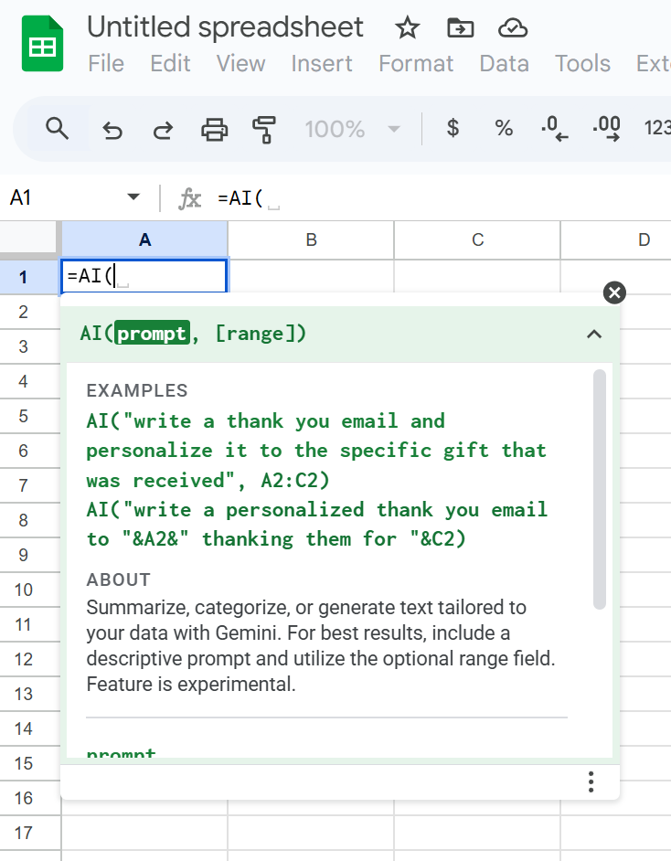
Prompt Gemini directly in your Sheets
Google Sheets now has a native AI function (often exposed as =AI() or =GEMINI(), depending on your Workspace rollout) that lets you talk directly to Google’s Gemini model from a cell.
Instead of nesting complex formulas, you can write natural-language prompts like:
=AI("Summarize this text in 3 bullet points:", A2)
You can use it to:
Summarize long text.
Classify or tag entries.
Extract key information from a sentence.
Generate content (subject lines, slogans, short paragraphs).
Because the prompt and the reference (like A2) live right in the formula, you can apply AI logic across a whole column just like any other function—without touching Apps Script or external tools.
If anything’s missing from this list, tell me! I’d love to hear your favourite Sheets tips and ideas.
Faster dashboards, cleaner code, and a rendering engine powered by the Sheets API.
Google Sheets is fantastic for quick dashboards, tracking tools, and prototypes. And with Apps Script, you can make them dynamic, automated, and even smarter.
But the moment you start building something real, a complex layout, a styled dashboard, a multi-section report, the Apps Script code quickly turns into:
messy
repetitive
slow
painful to maintain
Setting backgrounds, borders, number formats, writing values… everything requires individual calls, and your script balloon quickly.
To make this easier, you usually have two options:
Inject data into an existing template
Or…using RenderSheet
RenderSheet is a tiny, component-based renderer for Google Sheets, inspired by React’s architecture and built entirely in Apps Script. Let’s explore how it works.!
Introducing RenderSheet
RenderSheet is a lightweight, React-inspired renderer for Google Sheets.
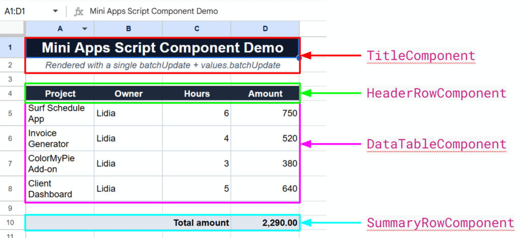
Instead of scattering .setValue(), .setBackground(), .setFontWeight(), etc. everywhere in your script, you write components:
<Title />
<HeaderRow />
<DataTable />
<SummaryRow />
<StatusPill />, etc.
Each component knows how to render itself. Your spreadsheet becomes a clean composition of reusable blocks, just like a frontend UI.
Why a “React-like” approach?
React works because it forces you to think in components:
a Header component
a Table component
a Summary component
a StatusPill component
Each component knows how to render itself, and the app becomes a composition of smaller reusable pieces.I wanted the exact same thing, but for spreadsheets.
With RenderSheet, instead of writing:
sheet.getRange("A1").setValue("Hello");
sheet.getRange("A1").setBackground("#000");
sheet.getRange("A1").setFontWeight("bold");
// and so on...
No direct API calls. No multiple setValue() calls. Just a clean render() method.
The Core Idea: One Render = Two Sheets API Calls
To achieve this “single render” effect, we simply divide to conquer:
one API call for injecting the data
and another for applying all the styling
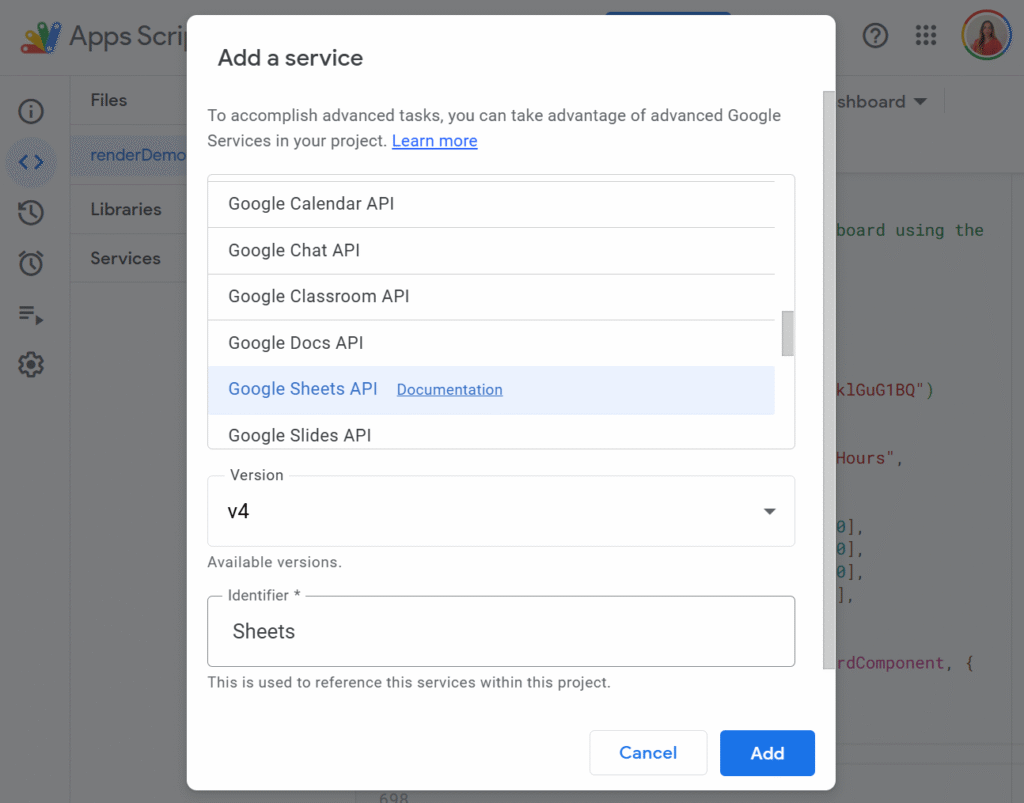
Before we can make the magic happen, we need to enable the Advanced Google Sheets API in our Apps Script project. This unlocks the batchUpdate method, the real engine behind RenderSheet.
To do so, just click the little + button on the left side panel, in front of Services, and select Google Sheets API:
This gives you access to the batchUpdate method, the real engine behind RenderSheet.
Now let’s look at the core mechanism.
The SheetContext (the Render Engine)
SheetContextis the core of RenderSheet. It collects all writes and formatting instructions and applies them in two API calls, using easy functions such as:
all data writes (writeRange)
all formatting instructions (setBackground, setTextFormat, setAlignment…)
But here’s the key:
None of these functions execute anything immediately. They only describe what the component wants to render.
The actual rendering only happens at the end, through two API calls.
You can think of SheetContext as your “toolbox”, and feel free to extend it with your own helpers.
Even though the initial setup is a bit more structured, the final result:
renders in 1 second
stays perfectly maintainable
allows components to be reused in any dashboard
Exactly the power of React, but in Google Sheets.
Final Thoughts
RenderSheet brings structure, speed, and clarity to Google Sheets development. If you’re tired of repetitive formatting code or want to build Sheets dashboards the same way you build UIs, this pattern completely changes the experience.
Let me know what you think, and feel free to contribute!
Even if I’m a real advocate of Apps Script, I’m also very aware of its limits when it comes to performance.
When a script keeps fetching the same API data or repeatedly processes large spreadsheets, things slow down fast. Each execution feels heavier than the previous one, and you end up wasting both user time and valuable API quota. Caching solves this problem by avoiding unnecessary work.
In this article, we’ll walk through what a cache actually is, how the Cache Service works in Apps Script, and the situations where it makes a real difference.
What’s a Cache?
A cache is simply a temporary storage area that keeps data ready to use. Instead of computing something again or fetching it every time, you store the result once, and reuse it for a short period.
For example, imagine calling an external API that takes half a second to respond. If you cache the result for five minutes, the next calls come back instantly. The data isn’t stored forever, just long enough to avoid waste.
This principle is everywhere in tech: browsers, databases, CDNs… and Google Apps Script has its own version too.
What Is Cache Service in Apps Script?
The Cache Service in Google Apps Script gives you a small, fast place to store temporary data. It comes in three “scopes” depending on your use case:
Data shared across all users of your script (getScriptCache)
Data specific to the current user (getUserCache)
Data linked to a particular document (getDocumentCache)
It only stores strings, which means that objects need to beserialized (JSON.stringify). The storage is also limited in size and duration: up to 100 KB per key, and a lifetime of up to 6 hours.
It’s not meant to replace a database or a sheet, it’s meant to speed up your script by avoiding repetitive or heavy work.
When Should You Use It?
Speeding up repeated API calls
If your script fetches data from GitLab, Xero, or any third-party API, calling that API every time is unnecessary. The Cache Service is ideal for storing the latest response for a few minutes. Your script becomes faster, and you avoid hitting rate limits.
Avoiding expensive spreadsheet reads
Large spreadsheets can be slow to read. If you always transform the same data (for example: building a dropdown list, preparing a JSON structure, or filtering thousands of rows), caching the processed result saves a lot of execution time.
Making HTMLService UIs feel instant
Sidebars and web apps built with HTMLService often reload data each time they open. If that data doesn’t need to be fresh every second, keeping it in cache makes the UI load instantly and improves the user experience noticeably.
Storing lightweight temporary state
For short-lived information—like a user’s last selected filter or a temporary calculation—Cache Service is much faster than PropertiesService, and avoids writing into Sheets unnecessarily.
A Simple Way to Use Cache Service
You can create a small helper function that retrieves data from the cache when available, or stores it if missing:
/**
 * Returns cached data or stores a fresh value if missing.
 * @param {string} key
 * @param {Function} computeFn Function that generates fresh data
 * @param {number} ttlSeconds Cache duration in seconds
 * @return {*} Cached or fresh data
 */
function getCached(key, computeFn, ttlSeconds = 300) {
  const cache = CacheService.getScriptCache();
  const cached = cache.get(key);
  if (cached) return JSON.parse(cached);

  const result = computeFn();
  cache.put(key, JSON.stringify(result), ttlSeconds);
  return result;
}
And use it like this:
function getProjects() {
  return getCached('gitlab_projects', () => {
    const res = UrlFetchApp.fetch('https://api.example.com/projects');
    return JSON.parse(res.getContentText());
  });
}
This approach is enough to dramatically speed up most Apps Script projects.
Final Thoughts
The Cache Service is small, simple, but incredibly effective if used well. It won’t store long-term data and it won’t replace a database, but for improving performance and reducing unnecessary work, it’s one of the easiest optimizations you can add to an Apps Script project.
If you want, I can help you write a second article with more advanced techniques: cache invalidation, dynamic keys, TTL strategies, and UI refresh patterns.
Dashboards feel magical when they react instantly to a selection, no scripts, no reloads, just smooth changes as you click a dropdown.
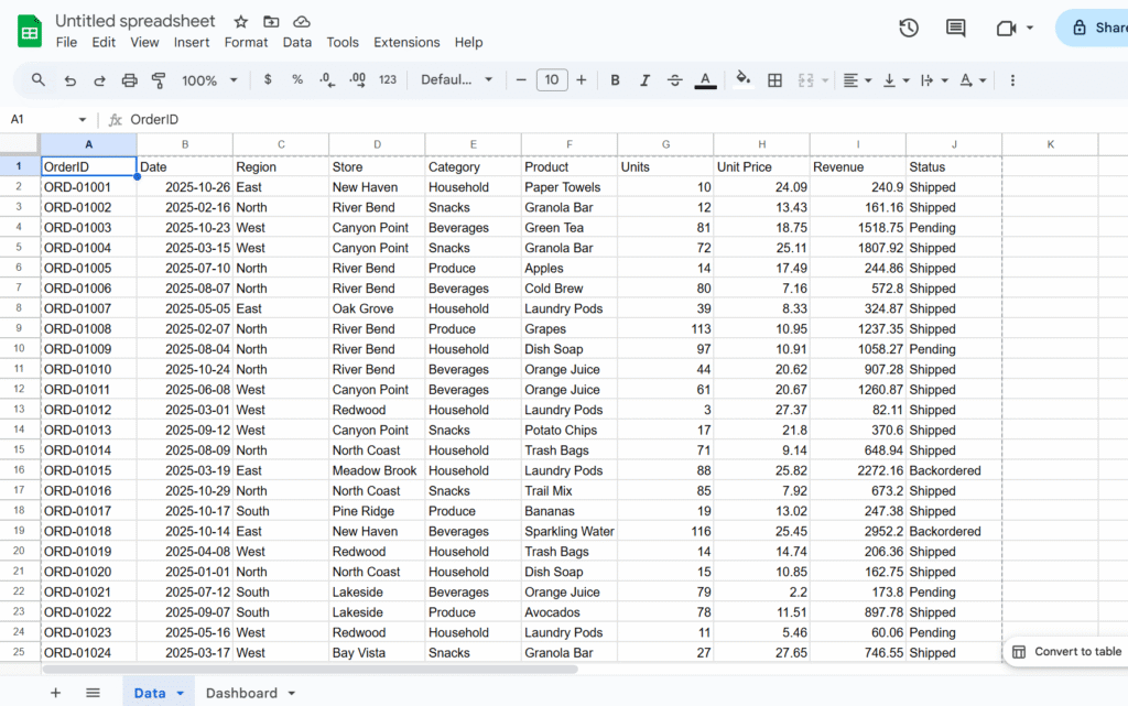
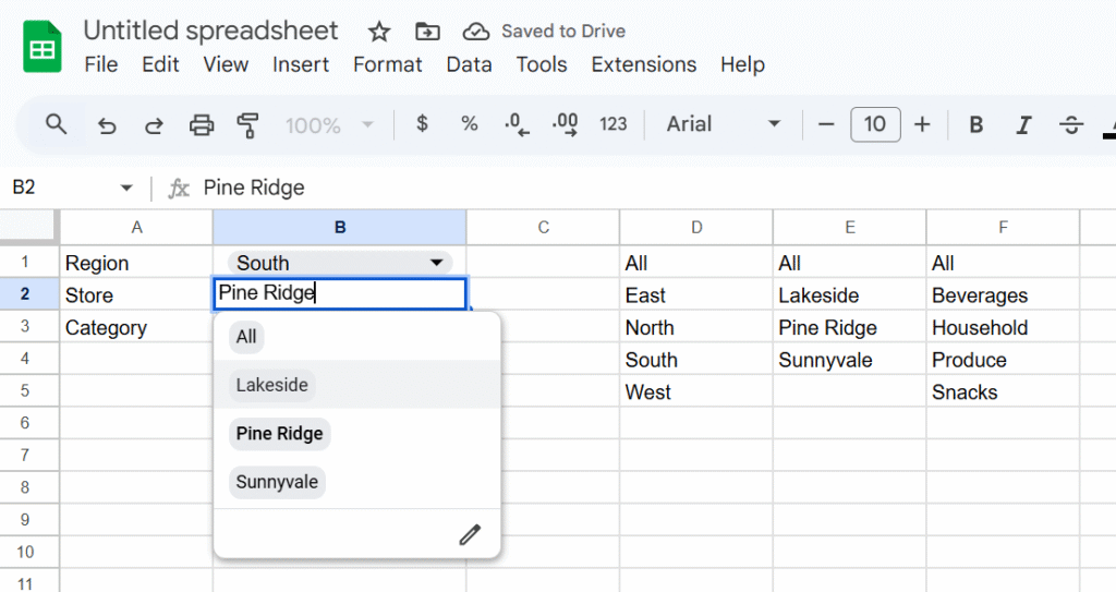
In this tutorial, we will build exactly that in Google Sheets: pick a Region, optionally refine by Store and Category, and watch your results table update in real time. We’ll use built-in tools, Data validation for dropdowns and QUERY for the live results, so it’s fast, maintainable, and friendly for collaborators.
In this example, we’ll use a sales dataset and create dropdowns for Region, Store, and Category, but you can easily adapt the approach to your own data and fields.
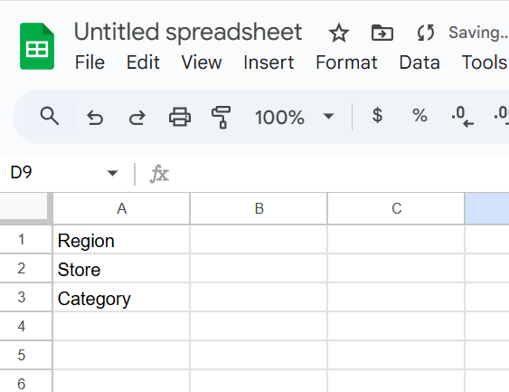
Step 1 – Add control labels
Let’s create a sheet, named Dashbaord, and add
A1:Region
A2:Store (dependent on Region)
A3:Category
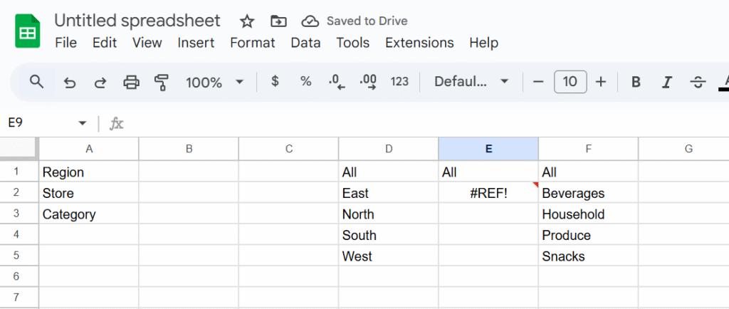
Step 2 – Build dynamic lists (helper formulas)
In column D, we will create a dynamic list of region with the following formula (insert the formula in D1):
Google Sheets is amazing, until it isn’t. As your spreadsheets grow with formulas, collaborators, and live data, they can get painfully slow. Here are all the tricks I’ve found to help my clients get better performances.
Why Google Sheets Get Slow
Too many formulas, especially volatile ones (NOW(), TODAY(), RAND())
Large datasets (thousands of rows/columns)
Repeated or redundant calculations
Overuse of heavy formulas or IMPORTRANGE, ARRAYFORMULA, QUERY…
Dozens of collaborators editing simultaneously
Conditional formatting or custom functions on big ranges
Quick Fixes to Speed Things Up
✔️ Tidy Up Your Formulas
Start by removing or replacing volatile functions like NOW() or RAND() with static values when you don’t need them to update constantly. Use helper columns to calculate something once and reference that instead of repeating logic across rows.
Use fixed ranges (A2:A1000) instead of full-column references. Every formula referencing A:A makes Google Sheets look at all 50,000+ possible rows, even if you’re only using 1,000.
✔️ Lighten the Load
Think of your sheet as a backpack: if it’s stuffed with years of unused data and unnecessary features, it’ll be slow to move. Delete unused rows and columns. Archive old data to separate files. Keep the main spreadsheet focused on what matters now.
✔️ Be Visual, Not Flashy
Conditional formatting, while beautiful, is a silent performance killer. Use it selectively and avoid applying rules to entire columns or rows. Likewise, go easy on charts and embedded images. Move your dashboards to a separate file if needed.
Apps Script and Heavy-Duty Sheets
When dealing with large spreadsheets, your scripting strategy matters. Google Apps Script offers two main interfaces: SpreadsheetApp and the advanced Sheets API. While SpreadsheetApp is easier to use, it becomes painfully slow with big datasets because it handles operations cell by cell.
Instead, for serious performance, we lean heavily on the Sheets API and its batchUpdate method. This allows us to push changes to many cells at once, minimizing round trips and drastically speeding up execution.
Here’s a simple example that injects data into a large range using the Sheets API, not SpreadsheetApp:
// Example of data
const data = [{
  "range": "A35",
  "values": [["TEST"]]
}];

/**
 * Write to multiple, disjoint data ranges.
 * @param {string} spreadsheetId The spreadsheet ID to write to.
 * @see https://developers.google.com/sheets/api/reference/rest/v4/spreadsheets.values/batchUpdate
 */
function writeToMultipleRanges(spreadsheetId, data, sheetName) {

  let ssGetUrl = `https://sheets.googleapis.com/v4/spreadsheets/${spreadsheetId}`
  let options = {
    muteHttpExceptions: false,
    contentType: 'application/json',
    method: 'get',
    headers: { Authorization: 'Bearer ' + ScriptApp.getOAuthToken() }
  };
  let ssGetresponse = JSON.parse(UrlFetchApp.fetch(ssGetUrl, options));
  let sheets = ssGetresponse.sheets;
  let rowCount = 0;
  let sheetId = 0;
  sheets.forEach(sheet => {
    if (sheet.properties.title == sheetName) {
      rowCount = sheet.properties.gridProperties.rowCount
      sheetId = sheet.properties.sheetId;
    }
  });

  let num = parseInt(String(data[0]["range"]).split("!")[1].replace(/[^0-9]/g, ''));
  if (rowCount < num) {
    let diff = num - rowCount;
    let resource = {
      "requests": [
        {
          "appendDimension": {
            "length": diff,
            "dimension": "ROWS",
            "sheetId": sheetId
          }
        }
      ]
    };
    let ssBatchUpdateUrl = `https://sheets.googleapis.com/v4/spreadsheets/${spreadsheetId}:batchUpdate`
    let options = {
      muteHttpExceptions: true,
      contentType: 'application/json',
      method: 'post',
      payload: JSON.stringify(resource),
      headers: { Authorization: 'Bearer ' + ScriptApp.getOAuthToken() }
    };
    let response = JSON.parse(UrlFetchApp.fetch(ssBatchUpdateUrl, options));
  }

  const request = {
    'valueInputOption': 'USER_ENTERED',
    'data': data
  };

  try {
    const response = Sheets.Spreadsheets.Values.batchUpdate(request, spreadsheetId);
    if (response) {
      return;
    }
    console.log('response null');
  } catch (e) {
    console.log('Failed with error %s', e.message);
  }
}

/**
 * Converts a row and column index to A1 notation (e.g., 3, 5 → "E3").
 *
 * @param {number} rowIndex - The 1-based row index.
 * @param {number} colIndex - The 1-based column index.
 * @returns {string} The A1 notation corresponding to the given indices.
 */
function getA1Notation(rowIndex, colIndex) {
  if (rowIndex < 1 || colIndex < 1) {
    throw new Error("Both rowIndex and colIndex must be greater than or equal to 1.");
  }
  let columnLabel = "";
  let col = colIndex;
  while (col > 0) {
    const remainder = (col - 1) % 26;
    columnLabel = String.fromCharCode(65 + remainder) + columnLabel;
    col = Math.floor((col - 1) / 26);
  }
  return columnLabel + rowIndex;
}
Freeze Formulas
Often, you only need a formula to calculate once, not every time the sheet updates.
Instead of leaving it active and recalculating endlessly, you can use Apps Script to compute the values once and then lock them in as static data.
The script below is designed for that: it keeps the original formulas in the second row (as a reference and for future recalculations), then copies those formulas down the column, computes all results, and finally replaces everything below the second row with raw values. The result? A faster sheet that still preserves its logic blueprint in row two.
/**
 *
 */
function Main_Update_Formula_Data(ssId, sheet) {

  // Get formulas in first row
  const formulas = sheet.getRange(2, 1, 1, sheet.getLastColumn()).getFormulas()[0];

  // Get last row index
  const lastRowIndex = sheet.getLastRow();

  // Prepare ranges to treat
  const ranges = [];

  // Loop through formulas to expand until the end
  for (let i = 0; i < formulas.length; i++) {

    if (formulas[i] != ""
      && !String(formulas[i]).startsWith("=arrayformula")
      && !String(formulas[i]).startsWith("=ARRAYFORMULA")
      && !String(formulas[i]).startsWith("=ArrayFormula")) {

      const thisRange = {
        startRowIndex: 1,
        endRowIndex: lastRowIndex - 1,
        startColumnIndex: i,
        endColumnIndex: i + 1,
        formulas: [formulas[i]],
      };

      ranges.push(thisRange);
    }
  }

  // Inject and freeze data except first row of formulas
  injectAndFreezeFormulas(ssId, sheet.getSheetId(), sheet.getName(), ranges);
}


/**
 * Injects formulas into multiple ranges, waits for computation, then replaces them with static values.
 * @param {string} spreadsheetId - Spreadsheet ID.
 * @param {number} sheetId - Numeric sheet ID.
 * @param {string} sheetName - Sheet name (for value reads/writes).
 * @param {Array<Object>} ranges - Array of range configs like:
 * @return {void}
 */
function injectAndFreezeFormulas(spreadsheetId, sheetId, sheetName, ranges) {
  // --- Inject formulas via batchUpdate
  const requests = [];
  ranges.forEach(rangeDef => {
    const {
      startRowIndex,
      endRowIndex,
      startColumnIndex,
      endColumnIndex,
      formulas,
    } = rangeDef;

    formulas.forEach((formula, idx) => {
      requests.push({
        repeatCell: {
          range: {
            sheetId,
            startRowIndex,
            endRowIndex,
            startColumnIndex: startColumnIndex + idx,
            endColumnIndex: startColumnIndex + idx + 1,
          },
          cell: {
            userEnteredValue: { formulaValue: formula },
          },
          fields: 'userEnteredValue',
        },
      });
    });
  });

  Sheets.Spreadsheets.batchUpdate({ requests }, spreadsheetId);
  Logger.log(`Formulas injected into ${ranges.length} range(s)`);

  // --- Wait briefly to ensure calculations are done
  Utilities.sleep(1000);

  // --- Read computed values via API (valueRenderOption: UNFORMATTED_VALUE)
  const readRanges = ranges.map(r =>
    `${sheetName}!${columnLetter(r.startColumnIndex + 1)}3:` +
    `${columnLetter(r.endColumnIndex)}${r.endRowIndex + 1}`
  );

  const readResponse = Sheets.Spreadsheets.Values.batchGet(spreadsheetId, {
    ranges: readRanges,
    valueRenderOption: 'UNFORMATTED_VALUE',
  });

  // --- Reinject values (overwrite formulas)
  const writeData = readResponse.valueRanges.map((vr, idx) => ({
    range: readRanges[idx],
    values: vr.values || [],
  }));

  Sheets.Spreadsheets.Values.batchUpdate(
    {
      valueInputOption: 'RAW',
      data: writeData,
    },
    spreadsheetId
  );

  Logger.log(`Formulas replaced by static values in ${writeData.length} range(s)`);
}

/**
 * Helper — Convert a column index (1-based) to A1 notation.
 *
 * @param {number} colIndex - 1-based column index.
 * @return {string}
 */
function columnLetter(colIndex) {
  let letter = '';
  while (colIndex > 0) {
    const remainder = (colIndex - 1) % 26;
    letter = String.fromCharCode(65 + remainder) + letter;
    colIndex = Math.floor((colIndex - 1) / 26);
  }
  return letter;
}
Did you know all of these tricks? If you’ve got a favorite performance tip, clever automation, or formula hack, drop it in the comments! Let’s keep our Sheets smart, fast, and fun to work with.