Filter by a Dropdown in Google Sheets (Data Validation + QUERY)

Dashboards feel magical when they react instantly to a selection, no scripts, no reloads, just smooth changes as you click a dropdown.

In this tutorial, we will build exactly that in Google Sheets: pick a Region, optionally refine by Store and Category, and watch your results table update in real time. We’ll use built-in tools, Data validation for dropdowns and QUERY for the live results, so it’s fast, maintainable, and friendly for collaborators.

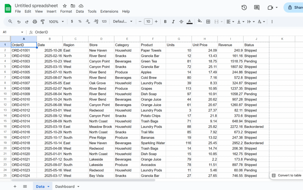
In this example, we’ll use a sales dataset and create dropdowns for Region, Store, and Category, but you can easily adapt the approach to your own data and fields.

Step 1 – Add control labels

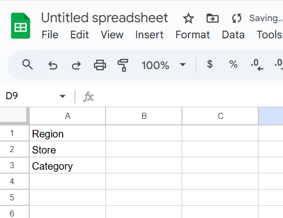
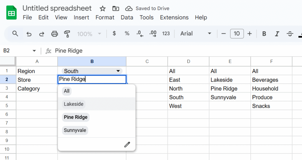
Let’s create a sheet, named Dashbaord, and add

Step 2 – Build dynamic lists (helper formulas)

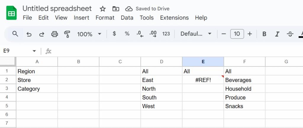
In column D, we will create a dynamic list of region with the following formula (insert the formula in D1):

={"All"; SORT(UNIQUE(FILTER(Data!C2:C, Data!C2:C<>"")))}

In column E, we will create a depending list for stores (changes when store update)

={"All";
  IF(Dashboard!B1="All",
     SORT(UNIQUE(FILTER(Data!D2:D, Data!D2:D<>""))),
     SORT(UNIQUE(FILTER(Data!D2:D, Data!C2:C=Dashboard!B1)))
  )
}

And in column F, the products

={"All"; SORT(UNIQUE(FILTER(Data!E2:E, Data!E2:E<>"")))}

Why formulas instead of manual lists? They stay in sync when new rows arrive.

Step 3 — Create the dropdowns (Data → Data validation)

=QUERY(
  Data!A1:J,
  "select * where (" &
    "(Col3 = '"&SUBSTITUTE(B1,"'","''")&"' or '"&B1&"'='All') and " &
    "(Col4 = '"&SUBSTITUTE(B2,"'","''")&"' or '"&B2&"'='All') and " &
    "(Col5 = '"&SUBSTITUTE(B3,"'","''")&"' or '"&B3&"'='All')" &
  ")",
  1
)

How it works

• The source range Data!A1:J sets column numbers for QUERY:
  • Col3 = Region, Col4 = Store, Col5 = Category.
• Each condition allows “All” to match everything.
• SUBSTITUTE(...,"'","''") safely escapes values like O'Brien.

If your headers aren’t in row 1, change the last parameter (1) to the correct header row count or adjust the range.

Hope this walkthrough helped! If there’s another Sheets topic you’d like me to cover, drop it in the comments.