Conditional formatting in Google Sheets is one of the easiest ways to make your data more readable and actionable. Instead of manually styling cells, you can automatically apply formatting based on rules.
Want to:
- Highlight values greater than 10
- Bold rows where status is “On going” and due date is today
- Instantly visualize trends
Conditional formatting handles all of that.
In this guide, you’ll learn the most useful techniques to master conditional formatting in Google Sheets.
How to add a conditional formatting rule in Google Sheets
To create a rule:
- Select your data range
- Go to Format → Conditional formatting
- The sidebar opens on the right, where you configure your rule
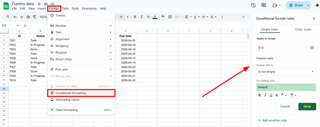
Let’s start with a simple example: highlight all statuses marked as “Done”.
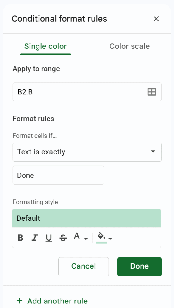
- Range: B2:B (this excludes headers and automatically includes new rows)
- Rule: Text is exactly →
"Done" - Formatting style: green background (you can also change text color, bold, etc.)
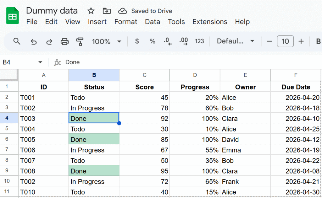
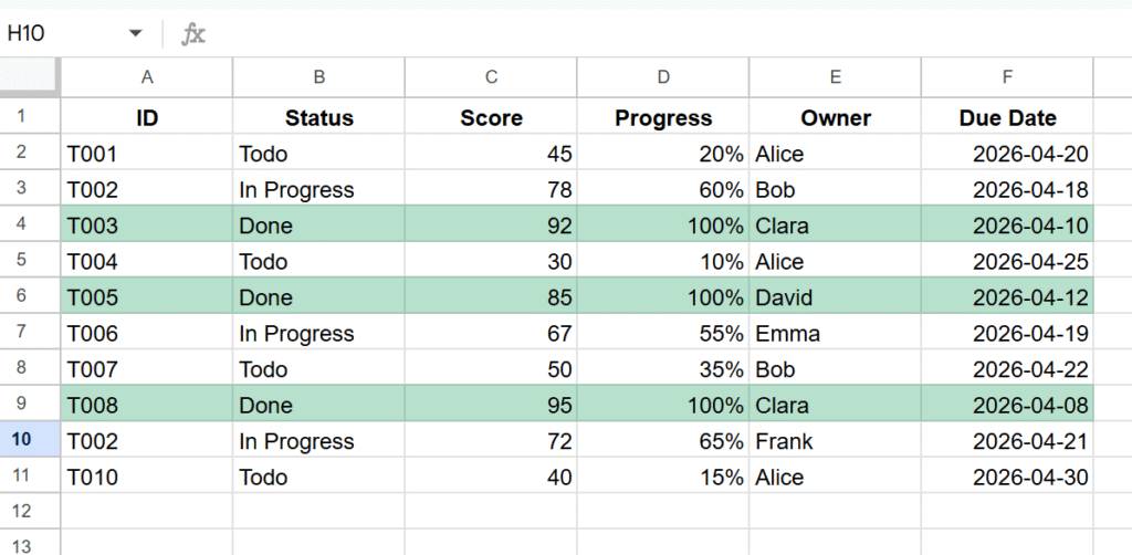
Apply conditional formatting to an entire row (custom formula)
In most cases, formatting a single cell is not enough. You often want to highlight the entire row based on a condition.
To do this, use a custom formula.
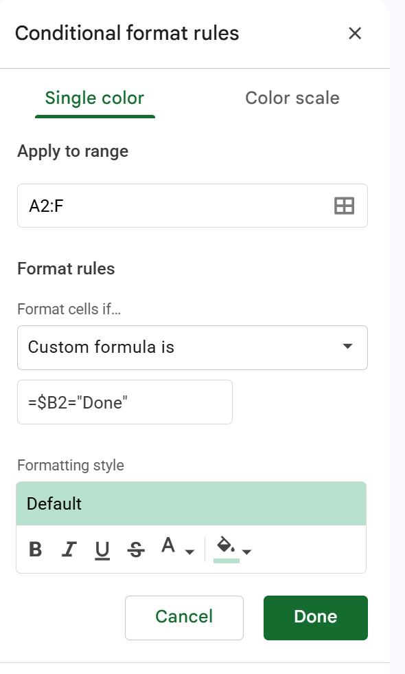
- Range: select your full dataset (e.g.
A2:E) - Format rule: Custom formula is
- Formula:
=$B2="Done"This formula checks column B (status), and if the value is “Done”, the formatting is applied to the entire row.
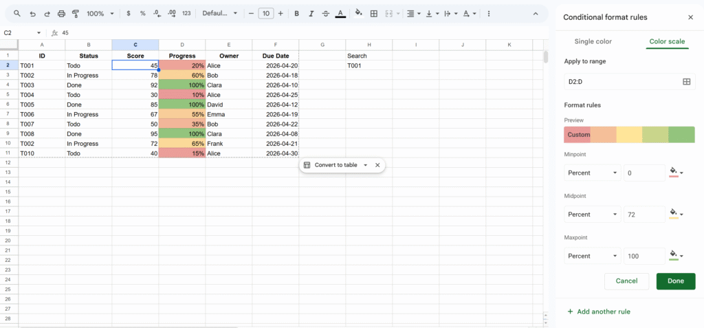
Use color scale for quick visual analysis
The color scale feature lets you apply a gradient based on numeric values.
You can access it from the second tab in the conditional formatting panel.
You can configure:
- The color gradient (low → high)
- Minimum, midpoint, and maximum values
- The type of values (number, percent, percentile)
Tip: Highlight duplicates in Google Sheets
A very common use case is detecting duplicates.
You can do this using a custom formula:
=COUNTIF($A$2:$A$100, A2) > 1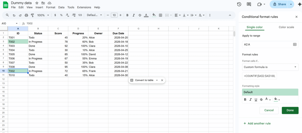
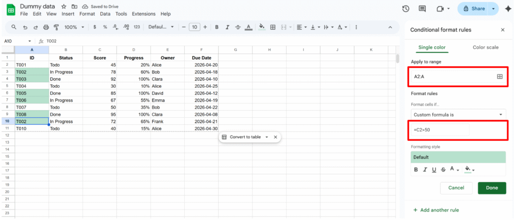
Tip: Format based on another cell
Conditional formatting doesn’t have to depend on the same cell. You can apply formatting based on values in another column.
For example, you can format column A depending on values in column B.
This approach is widely used in:
- Task trackers
- Workflow systems
- Status-based dashboards
The key is to combine ranges + custom formulas.
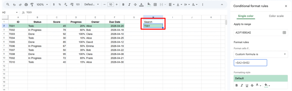
Tip: Highlight a row based on search input
You can also create a simple search experience directly in Google Sheets:
=$A2=$H$2- Cell
H2acts as a search input - When you type a value, matching rows are highlighted
This is very useful for:
- Quick lookups
- CRM systems
- Large datasets navigation
Final thoughts
This is a good base to understand how conditional formatting works.
Once you get the logic, you can easily adapt it to your own use cases and build more advanced rules.